Price Dynamics

In this chapter, we develop mathematical models to study the dynamics of asset prices over time. We begin with simple concepts of interests in discrete time capturing the time value of money. We then update the model to continuous time framework where an ordinary differential equation is obtained to describe the evolution of the deterministic price value under constant interest rate, ignoring the randomness. Finally, we extend the framework to stochastic models, where uncertainty in price movements is incorporated through a Wiener process. We also list some of the commonly used stochastic differential equations for stock prices and interest rates, which form the foundation of modern quantitative finance.

Deterministic Interest-rate Models

The interest, expressed as a percentage divided by 100, is referred to as the interest rate.

Typically, interest rates are calculated annually. In this section, we explore the theory of interest rates using a bank fixed deposit as an example of an investment tool. These concepts can be easily applied to other types of investment tools.

Let \(t\) denote the time variable. We consider \(t=0\) as the initial time of investment, and the investment period spans the interval \([0, T]\), where \(T > 0\) denotes the maturity time. The interest is paid at a certain frequency, representing the number of times interest is paid per annum. For example, if the interest is paid quarterly, the frequency is 4.

If the frequency of interest payments is denoted by \(m\), with \(n=mT\) being an integer, then the times at which interest payments are due are given by

\[ t_k = \frac{k}{m},\quad k=1,2,\ldots,n. \]

Let \(r\) denote the interest rate per annum (or annual interest rate), expressed as a decimal (i.e., \(r \times 100%\)). In this case, each interest payment is calculated at the rate \(r/m\), which is referred to as the per period rate.

Note:

Note that the phrase `per period' refers to each payment period \([t_{k-1}, t_k]\), for \(k=1,2,\ldots,n,\) whereas \([0,T]\) refers to the entire investment period. Observe that the per period rate \(r/m\) can be expressed as \(rT/n\).

Discrete Time Models

Let the principal be denoted by \(P(0)\) and the interest rate be \(r\) per annum. Let the payout frequency be \(m\) and the maturity time be \(T\), with \(n=mT\) being an integer. Let us derive the formula for compound interest.

At time \(t=t_1\), the accumulated amount is

\[ P(t_1) = P(0) \left(1+ \frac{r}{m}\right), \]

which is considered as the principal for the period \((t_1,t_2].\)

At time \(t=t_2\), we have

\[ P(t_2) = P(t_1) \left(1+ \frac{r}{m}\right) = P(0)\left(1+\frac{r}{m}\right)^2. \]

Continuing in this way, we see that

\[ P(t_k) = P(0)\left(1+\frac{r}{m}\right)^k, \quad k=1,2,\ldots, n. \]

In particular, at the maturity \(T\), the net amount obtained by the creditor (equivalently, the net amount paid by the debtor) is given by

\begin{eqnarray} P(T) = P(0)\left(1+\frac{r}{m}\right)^{n}, \end{eqnarray}

(2.1)

which is the nominal value or the future value of the investment with compound interest. The factor \(\left(1+\frac{r}{m}\right)^{n}\) is called the growth factor for compound interest.

Note:

The growth factor for compound interest can also be written as \(\left(1+\frac{rT}{n}\right)^{n}\).

When \(n=1\), we call the scheme a simple interest scheme.

Observe that the compound interest scheme is significantly influenced by the payout frequency \(m\). As the frequency increases, the maturity amount in the compound interest scheme also increases.

Example:

Mr. Megh invests ₹ 100 in a bank fixed deposit scheme at the rate of 10% per annum and for two and a half years. Assume that the bank pays out the interest every quarter. Then, the interest is paid 10 times to Mr. Megh with the interest payout frequency 4. Hence, we have \(m=4,\) whereas \(T=2.5,\) \(P(0)=100,\) and \(r=0.1\).

Using the compound interest formula, we can determine the accumulated amount at maturity (the nominal value), given by

\[ P(T) = 100\times\left(1+\frac{0.1}{4}\right)^{4\times 2.5} \approx 128. \]

Let us now increase the payout frequency from every quarter to every month, then we have \(m=12\) (instead of \(m=4\)) and the nominal value of the investment becomes

\[ P(T) = 100\times\left(1+\frac{0.1}{12}\right)^{12\times 2.5} \approx 128.27. \]

Hence the total interest obtained is ₹ 28.27, which is higher than the interest obtained with the quarterly compounding scheme.

Remark:

In the above example, we observe that, despite the interest rate being \(r=0.1\), ( i.e. 10%) per annum for two and a half years with quarterly compounding, the final interest obtained is ₹ 28. This amount is obviously more than 10% per annum with simple interest calculation. Thus, the nominal interest rate alone is not a clear indicator of the compounding effect. An equivalent way to express the amount of interest obtained is through the effective annual rate (EAR) (or effective interest rate), defined as the annual interest rate \(r_e\) such that

\[ P(0)\left(1 + r_e\right)^T = P(0)\left(1+\frac{r}{m}\right)^{n}. \]

Since \(n=mT\), the above expression can be rewritten as

\[ r_e = \left(1+\frac{r}{m}\right)^{m} - 1. \]

Using this formula, we can find the EAR in the above example as \(r_e \approx 0.1038\) (or 10.38%).

The basic annual interest rate (\(r=0.1\) in the above example) is termed the nominal annual rate (NAR) or simply the interest rate per annum or nominal interest rate.

Problem:

Find the EAR for the following schemes:

3% compounded monthly for one year.
18% compounded quarterly for one year.

Answer: 1. 3.04%. 2. 19.25%.

Continuous Time Model

The compound interest discussed above assumes discrete payout times with a finite payout frequency \(m\). However, in theoretical contexts, it is often necessary to model compounding in a continuous time framework, which can be achieved by taking \(m\rightarrow \infty\). This is equivalent to taking \(n\rightarrow \infty\) in (2.1) and leads to

\begin{eqnarray} P(T) = P(0) e^{rT}, \end{eqnarray}

(2.2)

the nominal value (or the future value) of the investment under continuous compound interest.

Example:

The nominal value of the fixed deposit offer given in Example «Click Here» using the continuous compound interest scheme is expressed as

\[ P(T) = 100\times e^{(0.1\times 2.5)} \approx 128.4. \]

Note:

To emphasize the distinction between continuous compounding and compounding with a finite frequency, the latter is often referred to as discrete compound interest. In our discussions, `compound interest' always refers to discrete compound interest.

Remark:

Observe that the growth in simple interest, compound interest, and continuous compound interest schemes is, respectively, the linear growth given by \(P(0)(1+rT)\), the geometric growth given by \(P(0)(1+r/m)^{mT}\) and the exponential growth given by \(P(0)e^{rT}\).

The factors

\[ A_s = (1+rT),\quad A_c = \left(1+\frac{r}{m}\right)^{mT}, ~\text{and}\quad A_{cc} = e^{rT} \]

are referred to as the accumulation factor for simple interest, compound interest, and continuous compound interest, respectively. The following figure illustrates the behavior of these three accumulation factors over time.

An illustration of accumulation factors

Problem:

Mr. Megh requires ₹ 10,000 exactly one year from today. He borrowed ₹ 10,00,000 from a friend with a commitment to repay the amount along with 4% continuously compounded interest after this one-year period. Now, he is exploring an opportunity to lend the borrowed money for one year in a simple interest scheme with an interest rate \(r\) to meet his financial need. Determine the approximate minimum value of \(r\).

\(~\)

Answer: \(r \approx 0.05081077\).

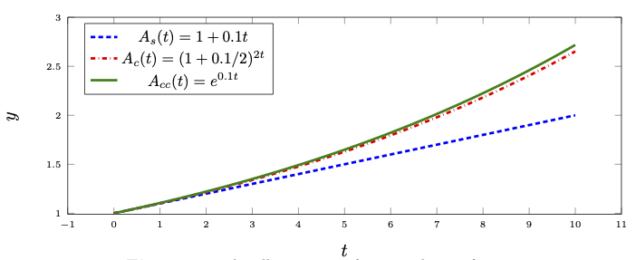
Often practitioners prefer continuous compounding interest rate in their models rather than discrete compounding interest rate. This may be because different markets often have different day count conventions. The following problem provides formulae to convert one interest rate to the other.

Problem:

Let \(r_d\) and \(r_c\) denote the discrete and continuous compound interest rates, respectively. If \(m\) is the payout frequency for the discrete compounding scheme and if the nominal value in both the schemes are equal at any maturity time, then show that

\[ r_c = m \ln\left(1+\frac{r_d}{m}\right) \quad \text{and}\quad r_d = m\left(e^{\frac{r_c}{m}} - 1\right). \]

Non-constant Interest Rate

We have derived the formula for continuous compounding in the case of a constant interest rate. However, a more realistic situation involves considering an interest rate that changes continuously over time. Hence, we need a model to calculate \(P(t)\) for all \(t \in [0,T]\), where \(r=r(t)\) represents the time-dependent interest rate.

We now derive an ODE that models the continuous compounding scheme with interest rate \(r=r(t)\) per annum at any given time \(t\in [0,T]\).

For a given number \(\Delta t>0\), the net interest obtain for the period \([t,t+\Delta t]\) is given by \(P(t+\Delta t) - P(t)\), for any \(t\in [0,T-\Delta t]\). Assume that \(\Delta t\) is very small so that the compound interest during the period \([t,t+\Delta t]\) is approximately the same as the simple interest. In other words, we take

\begin{eqnarray} P(t+\Delta t) - P(t) \approx r(t)\Delta t P(t). \end{eqnarray}

(2.3)

Dividing both sides by \(\Delta t\) and then letting \(\Delta t\rightarrow 0\), we get

\[ \lim_{\Delta t\rightarrow 0}\frac{P(t+\Delta t) - P(t) }{\Delta t} = r(t)P(t). \]

This leads to the required model, which is an ordinary differential equation (ODE) given by

\begin{eqnarray} \frac{dP}{dt} = rP. \end{eqnarray}

(2.4)

If we assume the interest rate \(r\) to be a constant, then the solution of (2.4) at \(t=T\), with the initial condition as the principal \(P(0)\), is given by (2.2).

Note:

By substituting (2.4) into (2.3), we observe that (2.3) is (approximately) the mean value theorem for \(P.\)

Integrating (2.4) over \([0,t]\), we can derive our required model as the integral equation

\begin{eqnarray} P(t) = P(0) + \int\limits_{0}^t r(s)P(s) ds. \end{eqnarray}

(2.5)

Using the fundamental theorem of calculus, we can see that if \(r\) and \(P\) are continuous, then (2.4) and (2.5) are equivalent.

Note:

The advantage of the model (2.5) over (2.4) is that (2.5) makes sense as long as \(r\) and \(P\) are integrable, whereas (2.4) requires both \(r\) and \(P\) to be continuous. Often, we come across a situation where \(r\) is not continuous and hence (2.5) is preferred in financial applications.

Problem:

Show, using the separation of variables method, that the particular solution of the ODE (2.4) at some time \(T>0\) is

\[ P(T) = P(0)e^{\int\limits_0^T r(t) dt}, \]

where the principle value \(P(0)\) is given.

Another important random phenomenon in finance is the mean-reverting process. Many natural and economic systems exhibit a mean-reverting tendency of a state variable (for instance, an interest rate), which can be described as follows:

Whenever the state variable deviates significantly from its long-term equilibrium (mean) level, forces arise that drive it back toward that mean.

Problem:

[Deterministic Mean-Reverting Model]

Show that the solution of the ODE

\[ dr_t = \lambda(\mu - r_t)dt. \]

\[ r_t = \mu + (r_0-\mu)e^{-\lambda t}. \]

By taking \(r(t)=r_t\), obtain the particular solution of the ODE (2.4) at some time \(T>0\).

The above problem shows the deterministic part of such dynamics and highlights the role of the stochastic part of mean-reverting models, which will be introduced at a later part of this chapter.

Present Value

So far, we have established models to calculate the nominal value \(P(T)\) of a deposit, given the principal \(P(0)\), interest rate \(r\), and the frequency \(m\) of the interest payment per year. Here \(P(T)\) can be regarded as the future value of the principal \(P(0)\) with respect to the given interest rate \(r\) and the frequency \(m\).

The concept of present value is the inverse of future value, where \(P(T)\) is given, and we are required to find \(P(0)\) for the given values of \(r\) and \(m\).

The present value with simple interest is given by

\[ P(0) = \frac{P(T)}{1+rT}. \]

In the case of a compound interest scheme, the present value is given by

\[ P(0) = P(T)\left(1+\frac{r}{m}\right)^{-n} = P(T)\left(1+\frac{rT}{n}\right)^{-n}, \]

where \(m\) denotes the frequency (the number of times interest is accumulated per annum) and \(n=mT\) is the total number of times interest is accumulated during the entire investment period.

Finally, for a continuous compounding scheme, the present value is given by

\[ P(0) = P(T) e^{-rT}. \]

The procedure of finding the present value for a future amount is referred to as discounting. Correspondingly, the present value is often referred to as discount value. The factor by which the present value \(P(0)\) is discounted from the future value \(P(T)\) is called the discount factor. The discount factor for simple interest, compound interest, and continuous compound interest are, respectively,

\begin{eqnarray} D_s = \frac{1}{1+rT},~~ D_c = \left(1+\frac{r}{m}\right)^{-mT}, \text{ and } D_{cc} = e^{-rT}. \end{eqnarray}

(2.6)

Note:

The concept of discounting plays an important role in pricing options because it provides a measure of the risk-free future value of money.

Cash Flow Stream

The concepts of present and future values can be extended to a sequence of cash flows occurring at multiple times. Let us first introduce the concept of a cash flow stream.

Definition:

[Cash Flow Stream]

For a given time partition \(\{t_0,t_1,\ldots,t_n\}\) of the period \([0,T]\) with \(0=t_0 < t_1 , the \textbfNI{cash flow stream} is represented by the \((n+1)\)-tuple \(\boldsymbol{x} = (x_0,x_1,\ldots,x_n)\), where \(x_k\), for \(k=0,1,\ldots,n\), denotes the value of money transacted at time \(t=t_k\).

Whenever the time partition is important, we may also represent a cash flow stream as (\(\boldsymbol{x},\boldsymbol{t}\)), where \(\boldsymbol{t} = (t_0,t_1,\ldots,t_n)\).

Note:

Generally, we set \(t_0=0\) as the initial investment time and \(t_n = T\) as the maturity time. A positive \(x_k>0\) indicates an inflow of money, while a negative \(x_k<0\) represents an outflow. If an entity holds the cash flow stream \(\boldsymbol{x}\), then the opposing party holds the cash flow stream \(-\boldsymbol{x}\), representing the exact opposite transactions.

Example:

Suppose Mr. Poor borrowed ₹ 1200 from his friend, Mr. Rich, and promised to pay ₹ 300 every quarter. If no interest charged, then the cash flow stream for Mr. Poor is \((1200, -300, -300, -300, -300),\) whereas the cash flow stream for Mr. Rich is given by \((-1200, 300, 300, 300, 300).\) If we denote the cash flow stream of Mr. Poor as \(\boldsymbol{x}\) and that of Mr. Rich as \(\boldsymbol{y}\), then we see that \(\boldsymbol{x} = -\boldsymbol{y}\).

Problem:

Consider the cash flow stream \((-100,3,3,3,103)\) into a bank, where transactions occur annually. Determine whether this represents a deposit received or a loan given by the bank. Additionally, find the annual rate of interest and identify the type of interest scheme ( i.e., whether it is simple interest or compound interest).

The future value of a cash flow stream \(\boldsymbol{x} = (x_0,x_1,\ldots,x_n)\) at the rate of \(r\) (per annum) during the time period \([0,T]\) with equally spaced time partition \(\{t_0,t_1,\ldots, t_n\}\) (with \(t_0=0\) and \(t_n=T\)) is given by

\begin{eqnarray} \text{FV}(\boldsymbol{x}) = \left\{\begin{array}{ll} \displaystyle{\sum_{k=0}^n} x_k\big(1+r(T-t_k)\big),&\text{ for simple interest},\\ \displaystyle{\sum_{k=0}^n} x_k\left(1+\frac{rT}{n}\right)^{n-k},&\text{ for compound interest,}\\ \displaystyle{\sum_{k=0}^n} x_k e^{r(T-t_k)},&\text{for continuous compound interest.} \end{array}\right. \end{eqnarray}

(2.7)

Note:

If \(m\) is the interest payout frequency per annum, then \(n=mT\). Thus the FV formula for compound interest is obtained by substituting \(m=n/T\) in (2.7).

Remark:

Define

\[ \tilde{r} = \frac{rT}{n}. \]

We can see that \(\tilde{r}\) represents the interest rate per period. Using \(\tilde{r}\) in the discrete compound interest formula, we get

\[ \text{FV}(\boldsymbol{x}) = \sum_{k=0}^m x_k\left(1+\tilde{r}\right)^{n-k}. \]

Note:

Depending on the given information about the interest rate ( i.e., whether it is the annual interest rate or interest rate per period), one has to choose the corresponding formula carefully.

Problem:

A depositor opted for a recurring deposit scheme in a bank, where she pays ₹ 1000 on the first day of every month, and for one year. Obtain the future value of the recurring deposit if the bank offers 6% annual interest with monthly compounding. Write the cash flow stream for the bank till the end of the scheme.

Answer: \(\boldsymbol{x}=(1000,1000,\ldots,1000, -12397.24)\)

Note:

One can easily obtain the formula for future value if the interest rate per period varies from period to period.

We now discuss the present value of a cash flow stream. Consider a cash flow stream \(\boldsymbol{x} = (x_0,x_1,\ldots,x_n)\). The present value of the cash flow stream \(\boldsymbol{x}\) at the interest rate of \(r\) per annum and for the time period \([0,T]\) with equally spaced time partition \(\{t_0,t_1,\ldots, t_n\}\) (with \(t_0=0\) and \(t_n=T\)) is given by

\[ \text{PV}(\boldsymbol{x}) = \sum_{k=0}^n x_k D_k, \]

where \(D_k\) denotes the discount factor at time \(t_k\) given by one of the formulae in (2.6) (with \(n=mT\)) depending on the type of the interest scheme. More precisely, we have

\begin{eqnarray} \text{PV}(\boldsymbol{x}) = \left\{\begin{array}{ll} \displaystyle{\sum_{k=0}^n} \frac{x_k}{1+rt_k},&\text{for simple interest},\\ \displaystyle{\sum_{k=0}^n} \frac{x_k}{\left(1+\dfrac{rT}{n}\right)^k},&\text{for compound interest},\\ \displaystyle{\sum_{k=0}^n} x_ke^{-rt_k},&\text{for continuous compound interest.} \end{array}\right. \end{eqnarray}

(2.8)

Note:

We always assume that, for a given cash flow stream \(\boldsymbol{x}=(x_0,x_1,\ldots, x_n)\), the number of times interest is paid or accumulated is \(n\). Unless otherwise stated, we assume a compound interest scheme where the interest due times coincide with the cash flow transaction times. Also, unless otherwise specified, we assume that in each period, interest is first accumulated, and then the transaction occurs.

Problem:

Determine the fair price of an annual cash flow stream \((0,50,50,50)\) for three years, given a prevailing compounding annual interest rate of \(r=0.08.\)

\(~\)

Answer: 128.8548

Note:

When the initial payment in a cash flow stream is zero (like the one given in the above problem), then we call the present value as the fair price of the cash flow stream. Whereas, if the initial payment is non-zero, then we refer the present value as the net present value (NPV).

Problem:

Find the net present value of the cash flow stream \(\boldsymbol{x} = (-10, 2, 3, 5, 2)\) if the prevailing per period interest rate is \(r=0.02\).

Answer: 1.4036

One can use present value to compare investments and prefer the one that yields higher value.

Example:

Consider a project where an initial amount of ₹ 5000 is invested in buying young goats that grow into marketable size within a year. After one year, the goats can either be sold for ₹ 7200 or left to grow further for an additional year, yielding better quality meat and higher demand, which can then be sold for ₹ 7600.

The corresponding cash flow streams are

\[ \boldsymbol{x_1} = (-5000,7200),~~\boldsymbol{x_2} = (-5000,0,7600). \]

If the prevailing interest rate is 6% per annum compounded annually, then which of the two cash flow streams is preferable?

To answer this question, let's calculate the net present value (NPV) for both streams. We have

\[ \text{NPV}(\boldsymbol{x_1}) = -5000 + \frac{7200}{1+0.06} \approx 1792.45,~~ \text{NPV}(\boldsymbol{x_2}) = -5000 + \frac{7600}{(1+0.06)^2} \approx 1763.97. \]

Therefore, based on the NPV criterion, it is more profitable to sell the goats at the end of the first year.

Problem:

Consider two annual cash flows

\[ \boldsymbol{x}_1 = (-13000, 5000, 6000, 7000) ~\text{ and }~ \boldsymbol{x}_2 = (-13000, 7000, 4800, 6000). \]

Answer the following questions with annual compound interest rates:

If \(r = 4.5%\), which cash flow is more profitable?
If \(r = 9%\), which cash flow is more profitable?

Remark:

[Uncountable Cash Flow Stream]

Often it is useful to consider an uncountable cash flow stream defined by a function \(f(t)\). The future value of such a cash flow stream under a constant interest rate \(r\) is given by

\[ \text{FV}(f) = \int\limits_0^T f(t)e^{r(T-t)}dt \]

and the present value is given by

\[ \text{PV}({f}) = \int\limits_0^T f(t)e^{-rt}dt. \]

The following example illustrates a potential application of a continuous cash flow stream and its present value.

Stochastic Models

Deterministic models discussed in the previous section captures the average or expected growth of financial variables such as prices or interest rates. However, real-world financial markets are inherently noisy and uncertain, and these variables are influenced by unpredictable factors such as news events, macroeconomic shocks, investor sentiments, and market reactions. Consequently, their dynamics cannot be modeled deterministically and to account this randomness, we extend our framework to include stochastic components, leading to stochastic differential equations (SDEs).

Stochastic Processes

In this subsection, we denote a financial variable by \(X\) (from our previous discussions, \(X\) can be the principal \(P\) or interest-rate \(r\)). In deterministic setup, \(X\) is viewed as a deterministic function of time \(X=X(t)\), where each time \(t\) corresponds to a single predictable value. However, in stochastic modeling, we abandon this deterministic view and treat \(X\) as a stochastic process.

Definition:

[Stochastic Process]

Let \(\mathbb{T}\) denote the time index set. A collection of random variables \(\{X_t~|~t\in \mathbb{T}\}\) defined on a probability space \((\Omega, \mathcal{F}, \mathbb{P})\) is called a stochastic process. If \(\mathbb{T}\) is an interval, then \(\{X_t\}\) is a continuous-time stochastic process and if \(\mathbb{T}\) is finite or countably infinite, then the process is a discrete-time stochastic process.

Note:

Often we use the notation \(X=\{X_t\}\), and view it as a function of two variables.

For a fixed time \(t\in \mathbb{T}\), \(X_t:\Omega\rightarrow \mathbb{R}\) is a random variable and we write
\[ X(\omega) = X_t(\omega), ~ \omega\in \Omega. \]
For a fixed random outcome \(\omega\in \Omega\), \(X:\mathbb{T}\rightarrow \mathbb{R}\) is a (deterministic) function of time,
\[ X(t) = X_t(\omega), ~t\in \mathcal{T}, \]
called a sample path of the process.

The time evolution of financial quantities inherently involve randomness, where the information unfolds progressively as events occur. This gradual flow of information is represented mathematically by the concept of filtration.

Definition:

[Filtration]

A collection \(\{\mathcal{F}_t~|~t\in \mathbb{T}\}\) of \(\sigma\)-fields on a sample space \((\Omega,\mathcal{F})\) is called a filtration if

\[ \mathcal{F}_s \subseteq \mathcal{F}_t \subseteq \mathcal{F},~{for all }0\le s\le t. \]

A probability space \((\Omega,\mathcal{F},\mathbb{P}, \{\mathcal{F}_t\})\) is called a filtered probability space.

Note:

The above definition is given in a general time framework. In discrete time, we have \(\mathbb{T} = \{t_0, t_1, \ldots\}\) (finite or infinite) and the corresponding filtration is denoted by \(\{\mathcal{F}_k~|~k=0,1,\ldots\}\).

In a finite horizon \([0, T]\) with partition \(\mathbb{T}_n = \{0=t_0, t_1, \ldots, t_n=T\}\), we often consider a filtration \(\{\mathcal{F}_k~|~k=0,1,\ldots, n\}\) with \(\mathcal{F}_n = \mathcal{F},\) the \(\sigma\)-field of the probability space (as obtained in Example «Click Here» ).

Often, filtrations are constructed using generated \(\sigma\)-fields, either from a partition of \(\Omega\) or from a stochastic process. These are the natural filtrations in financial applications. Here, we recall the definition of a generated \(\sigma\)-field by a partition of \(\Omega\) and postpone the discussion of \(\sigma\)-field generated by stochastic processes to a later chapter.

Definition:

[Generated \(\sigma\)-Field]

For a given collection of subsets \(\{E_1, E_2, \ldots \}\) (finite or infinite) of \(\Omega\), the generated \(\sigma\)-field, denoted by \(\sigma\{E_1, E_2, \ldots \}\), is defined as the intersection of all \(\sigma\)-fields on \(\Omega\) that contain the given collection. Equivalently, it is the smallest \(\sigma\)-field containing \(\{E_1, E_2, \ldots\}\).

Let us recall an elementary result from probability.

Problem:

Show that the generated \(\sigma\)-field, of a partition \(\texttt{P}\) of a set \(\Omega\), denoted by \(\sigma(\texttt{P})\), is the collection of all finite unions of the sets in \(\texttt{P}\) along with the empty set \(\emptyset\).

The following lemma is a direct consequence of the above problem.

Lemma:

For a given partition \(\mathbb{T}_n:=\{0=t_0,t_1,\ldots,t_n=T\}\) of \([0,T]\), let \(\{\texttt{P}_k~|~k=0,1,2\ldots, n\}\) be a sequence of partitions of \(\Omega\) such that \(\texttt{P}_{k+1}\) is finer than \(\texttt{P}_k\) for every \(k\in \{0,1,2,\ldots,n-1\}\). For each \(k\in \{0,1,2,\ldots,n\}\) if \(\mathcal{F}_k=\sigma(\texttt{P}_k)\), then the collection \(\{\mathcal{F}_k~|~k=0,1,\ldots, n\}\) is a filtration on \((\Omega, \mathcal{F}_n)\).

Each \(\sigma\)-field \(\mathcal{F}_t\) in a filtration can be interpreted as the collection of all information (about the market or a particular stock) that is available to an investor at time \(t\). This idea is illustrated in the following example.

Example:

[Discrete-Time Filtration in a Binomial Framework]

Given a pair of real numbers \(0 < B < 1 < U\). Consider a set of discrete time points \(\mathbb{T} = \{t_0, t_1, t_2\}\) and a sample space

\[ \Omega = \{\text{UU}, \text{UD}, \text{DU}, \text{DD}\}, \]

where each \(\omega=m_1m_2 \in \Omega\), with \(m_1,m_2\in \{U,D\}\), represents a possible sequence of a stock price movements at two time levels \(t_1\) and \(t_2,\) where U stands for an upward move and D represents a downward move.

Let us now choose a filtration that is relevant for the present problem.

At the initial time \(t_0\), no information is available. In order to reflect this, we choose the trivial \(\sigma\)-field

\[ \mathcal{F}_0 = \{ \emptyset, \Omega \}. \]

At time \(t_1\), the first movement (Up or Down) has been observed. Define

\[ E_1 = \{\text{UU}, \text{UD}\}, \quad E_2 = \{\text{DU}, \text{DD}\}. \]

The information available at \(t_1\) is then represented by the generated \(\sigma\)-field of the partition \(\{E_1, E_2\}\) of \(\Omega\). That is,

\[ \mathcal{F}_1 = \sigma\{E_1, E_2\} = \{ \emptyset, \Omega, E_1, E_2 \}. \]

At time \(t_2\), both movements have been observed, so the entire path is known. Thus, we define \(\mathcal{F}_2\) as the generated \(\sigma\)-field of the partition

\[ \{\text{UU}\}, \{\text{UD}\}, \{\text{DU}\}, \{\text{DD}\} \]

of \(\Omega\). That is,

\[ \mathcal{F}_2 = \sigma\{\{\text{UU}\}, \{\text{UD}\}, \{\text{DU}\}, \{\text{DD}\}\} = 2^\Omega. \]

Thus, the collection of \(\sigma\)-fields \(\{\mathcal{F}_0, \mathcal{F}_1, \mathcal{F}_2\}\) defined on \(\Omega\) satisfies the condition

\[ \mathcal{F}_0 \subset \mathcal{F}_1 \subset \mathcal{F}_2 = 2^\Omega, \]

and hence forms a filtration on the sample space \((\Omega, 2^\Omega)\). We refer to this filtration as the natural filtration for the binomial stock price process in discrete-time setup. This filtration represents the gradual flow of information over time, where as time progresses, the investor learns more about the realized path of the stock price.

The information structure described by a filtration is that the information increases in time and at any fixed time \(t\) an investor knows all information from the past to present but has no knowledge of future events. In financial terms, this expresses the no-insider-trading assumption: decisions at time \(t\) can depend only on currently available information.

In stochastic modeling, it is essential that the random quantities we study (such as stock prices, interest rates, or portfolio values) evolve consistently with the flow of information represented by the filtration. This needs another important concept called the adapted process.

Definition:

[Adapted Process]

A stochastic process \(\{X_t~|~t\in \mathbb{T}\}\) defined on a probability space \((\Omega, \mathcal{F},\mathbb{P})\) is said to be adapted to a filtration \(\{\mathcal{F}_t~|~t\in \mathbb{T}\}\) if \(X_t\) is \(\mathcal{F}_t\)-measurable, for every \(t\in \mathbb{T}\).

From the above definition, we see that an adapted process represents a realistic financial quantity whose evolution respects the market’s information structure.

Problem:

Let the initial stock price \(S_0>0\) at time \(t_0\) (present time) be known, and let the up and down factors be \(U=1.1\) and \(D=0.95\), respectively. For \(\mathbb{T} = \{t_0,t_1, t_2\}\), with \(t_1 < t_2\), consider the sample space \((\Omega, 2^\Omega)\), where \(\Omega\) is given in Example «Click Here» with \(UD = U\times D.\)

Let us use the notation \(\omega = m_1\times m_2\), for any \(\omega \in \Omega\), where each \(m_1, m_2\in \{U,D\}\). Define the stochastic process \(S = \{S_k~|~ t_k \in \mathbb{T}, ~k=1,2\}\) by

\[ S_1(\omega) = m_1S_0 , ~~ S_2(\omega) = (m_1\times m_2)S_0, ~\omega\in \Omega. \]

Show that \(S\) is adapted to the filtration \(\{\mathcal{F}_0, \mathcal{F}_1, \mathcal{F}_2\}\) constructed in Example «Click Here» .

In financial modeling, stochastic processes are used to describe quantities whose future values are uncertain, such as stock price or interest rates.

Stock Price Model

In this section, we derive a stochastic differential equation (SDE) governing the evolution of a stock price process, whose solution in known as the geometric Brownian motion. We also outline a computational procedure for simulating a stock price process.

Following the motivation from a previous Section «Click Here», let us take the deterministic part of the model as

\begin{eqnarray} \frac{dS_t}{dt} = \tilde{\mu} S_t, \end{eqnarray}

(2.9)

where \(\tilde{\mu}\), called the drift rate, is the average rate of return of the stock. This model provides a simple description of deterministic exponential price growth. Since stock prices evolve multiplicatively, it is suitable to model the logarithm of the price process rather than the price itself. So, let us consider the process

\[ X_t = \log\left(\frac{S_t}{S_0}\right). \]

Then, at the deterministic level, \(X_t\) satisfies the ODE

\[ dX_t = \tilde{\mu} dt. \]

We now extend the deterministic model by introducing randomness through an additive noise term, leading to the stochastic model

\begin{eqnarray} dX_t = \mu dt + {noise}, \end{eqnarray}

(2.10)

where the term `noise' represents the random fluctuation component to be characterized. Observe that we now use the notation \(\mu\) to denote the drift coefficient, representing the expected rate of change (or mean drift) of the stochastic process \(\{X_t\}\).

The basic idea of a stochastic model is to assume the noise term to be Gaussian white noise. In order to keep the mathematical discussion simple, we begin with a discrete-time approximation of Gaussian white noise.

Consider the partition of \([0,T]\) as

\[ \mathbb{T}_n = \{ t_0, t_1, \ldots, t_n \}, \quad t_k = k \Delta t, \quad \Delta t = \frac{T}{n}. \]

A discrete Gaussian white noise is a stochastic process \(\big\{\epsilon_t~|~t\in \mathbb{T}_n\big\}\) that satisfies the following properties for all \(j, k=0,1,\ldots, n-1\):

\(\epsilon_{t_k} \sim\mathcal{N}(0,\sigma^{2}_{\epsilon})\), for some constant \(\sigma^{2}_{\epsilon}>0\); and
the autocorrelation property \( \mathbb{E}[\epsilon_{t_j}\epsilon_{t_k}] = 0,\) for \( j \neq k.\)

Remark:

Often Property 2 is replaced by a stronger condition that \(\epsilon_t\) and \(\epsilon_s\) are independent for \(s\ne t\). Note that independence implies zero autocorrelation, but the converse need not hold. In what follows, we always assume that Gaussian white noise is an i.i.d process \(\{\epsilon_{t}\}\) such that \(\epsilon_t \sim\mathcal{N}(0,\sigma^{2}_{\epsilon})\), for some \(\sigma_\epsilon>0\).

Let us take \(\epsilon_{t_k}\sim\mathcal{N}(0,1)\) and define the discrete process

\[ W_{t_k} = \sqrt{\Delta t}\sum_{j=0}^{k-1} \epsilon_{t_j}, ~~ k=1,2,\ldots, n. \]

This process satisfies the recursive relation

\begin{eqnarray} W_{t_{k+1}} = W_{t_k} + \epsilon_{t_k}\sqrt{\Delta t}, ~~ k=0,1,\ldots, n-1 \end{eqnarray}

(2.11)

with \(W_0=0\), and the process \(\{W_{t_k}~|~k=0,1,\ldots, n\}\) is called a random walk.

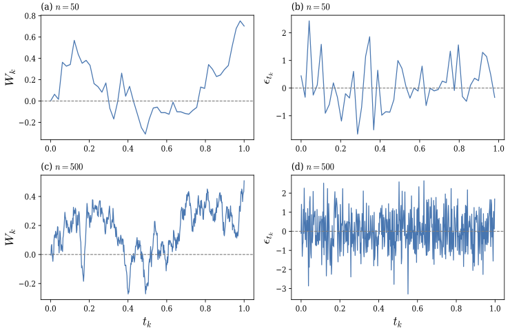
An illustration of the random walk (2.11) (a,c) and the corresponding discrete white noise (b,d) in the interval \([0,1]\).

The random walk and the corresponding discrete white noise are depicted in Figure «Click Here» for \(T=1\).

Wiener Process

For every \(j,k=0,1,\ldots,n,\) with \(j < k\), we can write

\[ W_{t_k} - W_{t_j} = \sum_{i=j}^{k-1} \epsilon_{t_i} \sqrt{\Delta t}, \]

which shows that \(W_k-W_j\) is a normally distributed random variable with

\[ E\big( W_{t_k} - W_{t_j}\big) = 0 ~~{and}~~ {Var}\big(W_{t_k} - W_{t_j}\big) = t_k - t_j. \]

Since \(\{\epsilon_{t_k}\}\) is an independent process, for any \(t_0\le t_{k_1} < t_{k_2} < t_{k_3}\le t_n\), the random variables \(W_{t_{k_2}} - W_{t_{k_1}}\) and \(W_{t_{k_3}} - W_{t_{k_2}}\) are independent because these random variables are sum of two distinct set of \(\epsilon\)'s which are themselves independent.

Now, we consider the limiting behaviour of the discrete-time process \(\{W_k\}\) as the time step \(\Delta t \to 0\). To obtain a continuous-time process on \([0,T]\), we define the piecewise linear interpolation

\[ W^{(n)}(t) = W_{t_k} + \frac{t - t_k}{\Delta t}\big(W_{t_{k+1}} - W_{t_k}\big), ~~ t \in [t_k, t_{k+1}),~~k=0,1,\ldots,n-1. \]

Thus, \(W^{(n)}(t)\) is a continuous, piecewise linear random function that satisfies (by (2.11), also see Figure «Click Here» (a,c))

\begin{eqnarray} W^{(n)}(t_{k+1}) - W^{(n)}(t_k) = \epsilon_{t_k}\sqrt{\Delta t}. \end{eqnarray}

(2.12)

By taking \(\Delta t\rightarrow 0\) (or equivalently, \(n \to \infty\)), the sequence of processes \(\{W^{(n)}(t)\}\) converges in distribution (weakly) in the space \(C[0,T]\) of continuous functions to a process \(\{W_t: t \in [0,T]\}\) and we write the expression (2.12) symbolically as

\[ dW_t = \epsilon_t \sqrt{dt}. \]

The process \(\{W_t\}\) obtained above is a Wiener process (or Brownian motion) as defined below.

Definition:

[Standard Brownian motion]

Let \((\Omega, \mathcal{F}, \mathbb{P}, \{\mathcal{F}_t\})\) be a filtered probability space. An adapted stochastic process \(\mathcal{W}=\{W_t~|~t\in [0,T]\}\) defined on this filtered probability space is called a standard Brownian motion (also known as a Wiener process) if it satisfies the following conditions:

Initial condition: \(W_0 = 0\) (\(\mathbb{P}\)-a.s).
Continuity property: For each \(s\in \Omega\), the map \(t\longmapsto W_t(s)\) from \([0,T]\) to \(\mathbb{R}\) is continuous. This is to say \(\mathcal{W}\) is a continuous stochastic process (\(\mathbb{P}\)-a.s is sufficient).
Independent increment property: For any partition \(t_0=0 < t_1 < t_2 < \ldots < t_n=T\), the random variables \(W_{t_1}\), \(W_{t_2}-W_{t_1}\), \(\ldots,\) \(W_{t_n} - W_{t_{n-1}}\) are independent.
Normal distribution: For each \(s,t\in [0,T]\) with \(s < t\), \(W_t-W_s\sim \mathcal{N}(0,t-s).\)

Note:

We omit the details and accept that the random walk process defined above tends to a Wiener process \(\{W_t~|~t\in [0,T]\}\) as \(\Delta t\rightarrow 0\). This convergence result follows from the celebrated Donsker’s invariance principle (or functional central limit theorem), which states that suitably scaled random walks converge in law to the Wiener process.

Remark:

Although the derivative \(\frac{dW_t}{dt}\) does not exist in the classical sense (because \(W_t\) is almost surely nowhere differentiable), the above differential relation is interpreted in the sense of Itô calculus, where \(dW_t\) represents an infinitesimal Gaussian increment with variance \(dt\).

In view of the above discussions, we propose to take the noise term to be proportional to \(dW_t\). Hence, we write the model (2.10) as

\begin{eqnarray} dX_t = \mu dt + \sigma dW_t, \end{eqnarray}

(2.13)

where \(\mu\) and \(\sigma>0\) are constants, and \(\{W_t\}\) is a Wiener process. This is a stochastic model, which is a stochastic differential equation. The process \(X=\{X_t\}\) governed by the above equation is called a generalized Wiener process with drift \(\mu\) and volatility \(\sigma\).

Problem:

Show, by a formal integration, that the solution of the equation (2.13) can be written in terms of the stock price process \(\{S_t\}\) as

\begin{eqnarray} S_t = S_0\exp\big(\mu t+\sigma W_t\big). \end{eqnarray}

(2.14)

Remark:

The drift coefficient \(\mu\) in the model (2.13) and in the solution (?) represents the instantaneous expected growth rate of the logarithmic return process \(\{X_t\}\).

On the other hand, the drift parameter \(\tilde{\mu}\) in the deterministic model (2.9) is interpreted as the expected rate of return (drift) of the stock process \(\{S_t\}\). The corresponding stochastic model for \(\{S_t\}\) is given by

\begin{eqnarray} dS_t = \tilde{\mu} S_t dt + \sigma S_t dW_t. \end{eqnarray}

(2.15)

The relation between \(\mu\) and \(\tilde{\mu}\) can be obtained using the Itô's formula (discussed below) and is given by

\begin{eqnarray} \tilde{\mu} = \mu + \frac{\sigma^2}{2}. \end{eqnarray}

(2.16)

Therefore, the stock price process \(\{S_t\}\) can also be expressed in terms of \(\tilde{\mu}\) as

\begin{eqnarray} S_t = S_0\exp\left(\left( \tilde{\mu} - \frac{\sigma^2}{2}\right)t+\sigma W_t\right) \end{eqnarray}

(2.17)

which is known as the geometric Brownian motion (GBM).

Itô Formula

As given in Remark «Click Here» , it is important to note that \(\mu=\tilde{\mu}\) holds only in deterministic models. In stochastic models, the presence of randomness alters the relationship between the drift of the price process and that of the log-price process, and hence \(\mu\) and \(\tilde{\mu}\) are generally different. This discrepancy arises because the classical chain rule of calculus is no longer valid for stochastic processes driven by Brownian motion. The appropriate replacement is given by Itô’s formula, which we discuss in this section in a general setting. We begin with the definition of an Itô process.

Definition:

[Itô process]

A stochastic process \(X=\{X_t\}\) is said to be an Itô process if it is governed by a stochastic differential equation of the form

\begin{eqnarray} dX = \mu(X,t) dt + \sigma(X,t) dW, \end{eqnarray}

(2.18)

where \(W\) represents a Wiener process, and both the drift and volatility are functions of \(X\) and \(t\).

From Remark «Click Here» , we see that the stock price process \(\{S_t\}\) is an Itô process. Further, we also derived an equation of the form given in the above definition for the process defined by \(X_t = \log(S_t/S_0)\). This shows that the process \(\{X_t\}\) is also an Itô process. The following lemma generalizes this result to any Itô process.

Lemma:

[Itô Lemma]

Let \(X\) be an Itô process of the form in Definition «Click Here» and let \(F=F(X,t)\), where \(F\in C^{2,1}(\mathbb{R}^2)\). Then, \(F\) is an Itô process satisfying the equation

\[ dF = \mu_F dt + \sigma_F dW, \]

where the drift and the volatility processes are given by

\begin{eqnarray} \mu_F &=& \frac{\partial F}{\partial t} + \mu \frac{\partial F}{\partial X} + \frac{\sigma^2}{2} \frac{\partial^2 F}{\partial X^2}, \\ \sigma_F &=& \sigma \frac{\partial F}{\partial X}. \end{eqnarray}

(2.19)

Note:

In the calculus of deterministic functions, the expression for \(\mu_F\) does not include the term \(\sigma^2 \frac{1}{2} \frac{\partial^2 F}{\partial x^2}.\)

Proof:

We omit the rigorous proof of the lemma and present only a formal derivation of the formula.

Let us take \(F=F(X,t)\), for \((X,t)\in \mathbb{R}^2\) and assume that \(F\) is smooth.

Using Taylor expansion, we can write

\begin{eqnarray} \Delta F = \frac{\partial F}{\partial X} \Delta X + \frac{\partial F}{\partial t} \Delta t + \frac{1}{2}\frac{\partial^2 F}{\partial X^2} \Delta X^2 + \frac{\partial^2 F}{\partial X\partial t} \Delta X \Delta t + \frac{1}{2}\frac{\partial^2 F}{\partial t^2} \Delta t^2 + \cdots \end{eqnarray}

(2.20)

Let us consider discrete form of the Itô process

\[ \Delta X = \mu(X,t) \Delta t + \sigma(X,t) \Delta W. \]

Since \(W\) satisfies the Wiener process, we have

\[ \Delta W= \epsilon \sqrt{\Delta t}. \]

Therefore, we have (dropping the arguments for the sake of notational convenience)

\[ \Delta X = \mu \Delta t + \sigma \epsilon \sqrt{\Delta t}, \]

Squaring both sides, we get

\[ \Delta X^2 = \sigma^2 \epsilon^2 \Delta t + o(\Delta t). \]

Substituting these expressions in (?), we get

\begin{eqnarray} \Delta F &=&\left( \mu \frac{\Delta F}{\Delta X} + \frac{\Delta F}{\Delta t}+ \frac{1}{2} \sigma^2 \frac{\Delta^2 F}{\Delta X^2} \epsilon^2 \right)\Delta t + \sigma \frac{\Delta F}{\Delta X}\Delta W + o(\Delta t). \end{eqnarray}

(2.21)

Since \(\epsilon \sim \mathcal{N}(0,1),\) we have

\[ \mathbb{E}(\epsilon^2 \Delta t) = \Delta t, ~~ \operatorname{Var}(\epsilon^2 \Delta t) = 2\Delta t^2. \]

Hence, we see that \(\epsilon^2 \Delta t - \Delta t \xrightarrow[]{~\text{m.s.}~} 0,\) as \(\Delta t\rightarrow 0\). This allows us to write

\[ \epsilon^2 \Delta t = \Delta t + o(\Delta t) ~~ (\text{in probability}),~ \text{as}~\Delta t\rightarrow 0. \]

Substituting this in the above expression for \(\Delta F\), neglecting \(o(\Delta t)\) terms and then taking \(\Delta t\rightarrow 0\), we get

\[ dF =\left( \mu \frac{\partial F}{\partial X} + \frac{\partial F}{\partial t}+ \frac{1}{2}\sigma^2\frac{\partial^2 F}{\partial X^2} \right)d t + \sigma \frac{\partial F}{\partial X}d W. \]

Problem:

Let \(S = \{S_t\}\) satisfies the SDE

\[ dS_t = \tilde{\mu} S_t dt + \sigma S_t dW_t, \]

for some given \(S_0>0.\) Define the process \(X=\{X_t\}\) by \(X_t = \log(S_t/S_0)\). Show that \(X\) is an Itô process and find its drift and volatility.

Parameter Calibration

In order to simulate the stock price process numerically using GBM given by the formula

\begin{eqnarray} S_t = S_0\exp\left(\left( \tilde{\mu} - \frac{\sigma^2}{2}\right)t+\sigma W_t\right), \end{eqnarray}

(2.22)

we need to estimate the model parameters, namely, the drift \(\tilde{\mu}\) (or equivalently \(\mu= \tilde{\mu} - \tfrac{1}{2}\sigma^2\)) and the volatility \(\sigma>0\). This process of determining the model parameter values from historical data is referred to as parameter calibration.

In this section, we obtain the empirical estimate of \(\mu\), denoted by \(\widehat{\mu}\) and \(\sigma\), denoted by \(\widehat{\sigma}\).

Given stock price observations \(\{S_k~|~k=0,1,\ldots, N\}\) at equally spaced times \(t_k = k\,\Delta t\), define the log-returns

\[ r_k = \ln\!\left(\frac{S_k}{S_{k-1}}\right),~~k=1,2,\ldots, N. \]

The empirical estimators \(\widehat{\mu}\) of the drift \(\mu\) of the log-return process can be obtained as

\[ \widehat{\mu} = \frac{1}{\Delta t} \left(\frac{1}{N}\sum_{k=1}^N r_k\right). \]

The empirical estimate \(\widehat{\sigma}\) of the volatility \(\sigma\) is obtained from the relation

\[ \widehat{\sigma}^2 = \frac{1}{(N-1)\,\Delta t}\sum_{k=1}^N (r_k - \overline{r})^2, \]

where \(\overline{r}\) denotes the sample mean of \(\{r_k\}\).

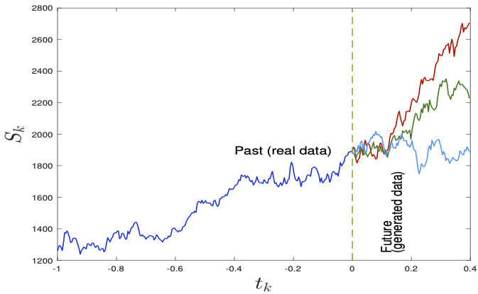
The stock price process using the GBM can now be simulated using the formula (2.22) with the estimated drift and volatility, given by

\begin{eqnarray} \widehat{S}_k = \widehat{S}_{k-1}\exp\left( \widehat{\mu} \Delta t + \widehat{\sigma} \epsilon_k \sqrt{\Delta t}\right), ~~ k=N+1, N+2, \ldots, \end{eqnarray}

(2.23)

where \(\epsilon_k \sim \mathcal{N}(0,1).\)

The following figure depicts three sample paths simulated using the calibrated GBM formula (2.23), with \(\Delta t = 1/252\) (a standard convention for the number of trading days per year).

One year daily closing price of Infosys Technology (labeled Past) and the stock price process (labeled Future) simulated using the calibrated GBM formula (2.23).

Code:

Write a python code to simulate 3 sample paths using the calibrated GBM formula (2.23) for a given time series data. You may get the data used in the simulation of the above figure from the following link: Daily closing price of Infosys

Interest-rate Models

In the previous subsection, we introduced a stochastic model for the stock price process based on a multiplicative growth criterion, leading to exponential behavior in the absence of random fluctuations. In this section, we introduce a stochastic model for the interest-rate process based on the mean-reverting phenomenon, which describes a process that tends to revert toward a long-term average level.

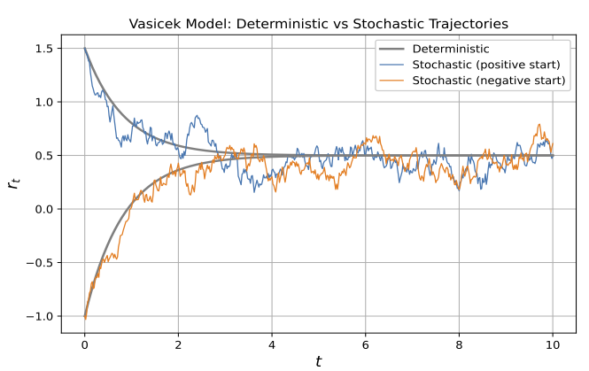
Recall that the deterministic version of the mean-reverting model was introduced in Problem «Click Here» . by including a stochastic component driven by Brownian motion, we obtain the stochastic model for the interest-rate process \(\{r_t\}\) as

\begin{eqnarray} dr_t = \lambda (\mu - r_t) dt + \sigma dW_t, \end{eqnarray}

(2.24)

where \(\lambda>0\) is the speed of mean reversion, \(\mu\) is the long-term mean level, and \(\sigma\) is the volatility (standard deviation) of random fluctuations.

This model is known as the Vasicek model in the financial context, especially for modeling the short-term interest-rate. Mathematically, the process \(\{r_t\}\) follows an Ornstein--Uhlenbeck process, a Gaussian mean-reverting stochastic process originally introduced in statistical physics.

The Vasicek model (2.24) is a linear SDE, which can be written in the linear form as

\[ dr_t + \lambda r_t\,dt = \lambda \mu\,dt + \sigma\,dW_t. \]

Multiplying both sides by the integrating factor \(e^{\lambda t}\) and using Itô lemma, we can rewrite the above equation equivalently as

\[ d\!\left(e^{\lambda t} r_t\right) = \lambda \mu e^{\lambda t}\,dt + \sigma e^{\lambda t}\,dW_t. \]

Integrate both sides from \(0\) to \(t\) gives

\[ e^{\lambda t} r_t - r_0 = \int_0^t \lambda \mu e^{\lambda s}\,ds + \int_0^t \sigma e^{\lambda s}\,dW_s. \]

Multiplying both sides by \(e^{-\lambda t}\), we obtain the exact solution of the Vasicek (Ornstein--Uhlenbeck) process as

\begin{eqnarray} r_t = r_0 e^{-\lambda t} + \mu(1 - e^{-\lambda t}) + \sigma \int_0^t e^{-\lambda(t-s)}\,dW_s. \end{eqnarray}

(2.25)

The first two terms represent the deterministic mean-reverting component, while the third term represents the stochastic contribution driven by the Wiener process and is expressed as a stochastic integral, which in this case is a Wiener integral because the integrand is a deterministic function.

Observe that, unlike the stock price process governed by the GBM, the exact solution (2.25) for the process \(\{r_t\}\) cannot be used directly to generate (or plot) simulated data, even when the parameters are given (or calibrated). This is because of the presence of the stochastic integral \(\int_0^t e^{-\lambda(t-s)}\,dW_s\), which is a random variable depending on the entire Brownian path \(\{W_t~|~t\in [0,1]\}\). Thus, the process \(\{r_t\}\) is known only in law (i.e., through its distribution), but not as an explicit function of time.

Wiener Integral

From the above discussion, it is clear that to simulate (or even interpret) the process \(\{r_t\}\), we must first understand how to define and evaluate a Wiener integral.

Let \(\{W_t\}_{t\ge 0}\) be a Wiener process defined on a probability space \((\Omega,\mathcal{F},\mathbb{P})\).

Step 1: Definition for step functions. Let \(f:[0,T]\to\mathbb{R}\) be a step function of the form

\[ f(t) = \sum_{k=0}^{n-1} a_k {1\hspace{-0.09in}1}_{(t_k,t_{k+1}]}(t), \qquad 0=t_0 < t_1 < \cdots < t_n=T, \]

where \(a_k\in\mathbb{R}\) are constants. The Wiener integral of \(f\) with respect to \(W_t\) is defined as

\[ \int_0^T f(t)\,dW_t := \sum_{k=0}^{n-1} a_k \bigl(W_{t_{k+1}}-W_{t_k}\bigr). \]

Problem:

[Isometry Property for Step Functions]

Show that for any step function \(f\),

\[ \mathbb{E}\!\left[\left(\int_0^T f(t)\,dW_t\right)^2\right] = \int_0^T f(t)^2\,dt. \]

Step 2: Extension to square-integrable functions. Let \(f\in L^2([0,T])\). Consider a uniform partition of \([0,T]\) in the form

\[ 0 = t_0^{(n)} < t_1^{(n)} < \cdots < t_n^{(n)} = T, ~~ t_k^{(n)} = \frac{kT}{n},~~ k=0,1,\ldots, n. \]

Define a sequence of step functions

\[ f_n(t) := \sum_{k=0}^{n-1} f\!\left(t_k^{(n)}\right)\, {1\hspace{-0.09in}1}_{(t_k^{(n)},\, t_{k+1}^{(n)}]}(t). \]

Problem:

Show that the sequence \(\{f_n\}\) given above satisfies

\[ \int_0^T |f_n(t)-f(t)|^2\,dt \;\longrightarrow\; 0. \]

Definition:

[Wiener Integral]

Let \(f\in L^2([0,T])\) and let \(\{f_n\}\) be a sequence of step functions such that

\begin{eqnarray} \int_0^T |f_n(t)-f(t)|^2\,dt \;\longrightarrow\; 0. \end{eqnarray}

(2.26)

The Wiener integral of \(f\) with respect to the Wiener process \(\{W_t\}\) is defined as

\begin{eqnarray} \int_0^T f(t)\,dW_t \;:=\; \lim_{n\to\infty} \int_0^T f_n(t)\,dW_t, \end{eqnarray}

(2.27)

where the limit is taken in the mean-square sense, that is,

\[ \lim_{n\to\infty} \mathbb{E}\!\left[ \left| \int_0^T f_n(t)\,dW_t - \int_0^T f(t)\,dW_t \right|^2 \right] =0. \]

The isometry property of the Wiener integral for step functions can be extended to \(L^2\)-functions.

Problem:

[Isometry Property for \(L^2\)-Functions]

Let \(\{W_t\}_{t\ge 0}\) be a Wiener process. Show that for any deterministic function \(f\in L^2([0,T])\), the Wiener integral satisfies the isometry property

\[ \mathbb{E}\!\left[ \left( \int_0^T f(t)\,dW_t \right)^2 \right] = \int_0^T f(t)^2\,dt. \]

Remark:

Since the integrand \(f\) is deterministic and belongs to \(L^2([0,T])\), the Wiener integral is a Gaussian random variable with

\[ \int_0^T f(t)\,dW_t \sim \mathcal{N}\!\left(0,\;\int_0^T f(t)^2\,dt\right). \]

The above result can be proved easily when the integrand \(f\) is a step function, and this case is left as an exercise. The proof for general \(f\in L^2([0,T])\) is omitted.

Numerical Simulation

We now discuss an exact numerical procedure to simulate the discrete-time mean-reverting process \(\{r_{t_k}\}_{k=0}^N\), for a partition

\[ 0=t_0 < t_1 < \cdots < t_N=T, \qquad \Delta t = t_{k+1}-t_k = \frac{T}{N}, \]

where \(N>0\) is a given integer.

The Wiener integral in (2.25) at \(t=t_{k+1}\) can be written as

\begin{eqnarray} \int_0^{t_{k+1}} e^{-\lambda(t_{k+1}-s)}\,dW_s &=& \int_0^{t_k} e^{-\lambda(t_{k+1}-s)}\,dW_s + \int_{t_k}^{t_{k+1}} e^{-\lambda(t_{k+1}-s)}\,dW_s\\ &=& e^{-\lambda\Delta t} \int_0^{t_k} e^{-\lambda(t_k-s)}\,dW_s + \int_{t_k}^{t_{k+1}} e^{-\lambda(t_{k+1}-s)}\,dW_s. \end{eqnarray}

(2.28)

Substituting the above expression in (2.25) gives the exact recursion relation

\begin{eqnarray} r_{t_{k+1}} = \mu + (r_{t_k}-\mu)e^{-\lambda\Delta t} + \sigma \int_{t_k}^{t_{k+1}} e^{-\lambda(t_{k+1}-s)}\,dW_s. \end{eqnarray}

(2.29)

Distribution of the stochastic increment

The integrand

\begin{eqnarray} s \mapsto e^{-\lambda(t_{k+1}-s)} \end{eqnarray}

(2.30)

is deterministic and belongs to \(L^2([t_k,t_{k+1}])\). Hence by Remark «Click Here» , the stochastic integral in (2.29) is a centered Gaussian random variable.

By the isometry property Problem «Click Here» , we have

\begin{eqnarray} \begin{aligned} \mathbb{E}\!\left[ \left( \int_{t_k}^{t_{k+1}} e^{-\lambda(t_{k+1}-s)}\,dW_s \right)^2 \right] &= \int_{t_k}^{t_{k+1}} e^{-2\lambda(t_{k+1}-s)}\,ds \\ &= \frac{1-e^{-2\lambda\Delta t}}{2\lambda}. \end{aligned} \end{eqnarray}

(2.31)

Therefore,

\begin{eqnarray} \int_{t_k}^{t_{k+1}} e^{-\lambda(t_{k+1}-s)}\,dW_s \sim \mathcal{N}\!\left( 0,\;\frac{1-e^{-2\lambda\Delta t}}{2\lambda} \right). \end{eqnarray}

(2.32)

Exact simulation scheme

Let \(\{Z_k\}_{k=0}^{N-1}\) be independent standard normal random variables, \(Z_k\sim\mathcal{N}(0,1)\). Then, we can write

\begin{eqnarray} \int_{t_k}^{t_{k+1}} e^{-\lambda(t_{k+1}-s)}\,dW_s = \sqrt{\frac{1-e^{-2\lambda\Delta t}}{2\lambda}}\; Z_k. \end{eqnarray}

(2.33)

Substituting into (2.29) yields the exact numerical scheme:

\begin{eqnarray} r_{k+1} = \mu + (r_k-\mu)e^{-\lambda\Delta t} + \sigma \sqrt{\frac{1-e^{-2\lambda\Delta t}}{2\lambda}}\; Z_k, \qquad Z_k\sim\mathcal{N}(0,1). \end{eqnarray}

(2.34)

Note:

\(~\)

The scheme (2.34) uses the exact transition distribution of the Vasicek model and therefore introduces no discretization bias.

The following figure depicts the numerical simulation of the mean-reverting process using the formula (2.34).

Numerical simulation of the mean-reverting process using (2.34).

Code:

Understand the python code given in the following link: Vasicek