Chapter 4: Network and Gradient Evaluation

In the last two chapters, we have studied models based on single neurons and observed the limitations in their applicability and expressivity. This clearly motivates the use of an artificial neural network as a model, especially when dealing with high-dimensional datasets involving more complex features. Our next task is, therefore, to understand the technique of training a multilayer perceptron (MLP).

As mentioned in Section 1.4, training or learning an MLP means obtaining suitable parameters \(\boldsymbol{\Theta}\) involved in defining the neural network function \({\mathscr{F}_{L,\hat{n}}}(\cdot\,; \boldsymbol{\Theta})\). The learning needs a suitably chosen cost function that is minimized using a gradient-based optimization method to obtain the parameters. To this end, we need to compute the gradient of the cost function, which uses the quantities generated while evaluating the neural network function at a given feature.

Recall from Chapter 1 that we have defined an MLP as a composition of layers of affine and activation functions (see Remark 1.1). A convenient and computationally efficient way of evaluating the neural network function at a feature \(\boldsymbol{x}\) is to consider each layer function in matrix form. The gradients are evaluated following the backpropagation technique. The purpose of this chapter is to set the matrix notation for the neural network function and understand the evaluation of the gradients of a cost function with respect to the parameters using repeated application of the chain rule across the layers.

The evaluation of a neural network function at a batch of features, given the set of parameters, is referred to as a batch forward propagation and is detailed in Section 4.1. The backpropagation method for gradient computation is detailed in Section 4.2.

4.1 Matrix Formulation and Forward Propagation

From Definition 1.2, we see that an ANN is defined as a composition of layers, where each layer applies an affine transformation followed by a nonlinear activation function. In this section, we first give matrix form of a neural network function and then discuss the batch forward propagation.

4.1.1 Layer Function in Matrix Form

In order to keep the notations clear and simple we use a shallow network with one hidden layer, that is, \(L=2\).

Let the network dimensions be \(n_0, n_1, n_2\in \mathbb{N}\). From Definition 1.2, a shallow network with width \(\hat{n}=n_1\) is a function \({\mathscr{F}_{2,\hat{n}}}:\mathbb{R}^{n_0}\rightarrow \mathbb{R}^{n_2}\) given by

\begin{eqnarray} {\mathscr{F}_{2,\hat{n}}} (\boldsymbol{x};\boldsymbol{\Theta}) = \mathfrak{h}^{(2)}\big(\mathfrak{h}^{(1)} (\boldsymbol{x};\overline{W}^{(1)});\overline{W}^{(2)}\big),~\boldsymbol{x}\in \mathbb{R}^{n_0}. \end{eqnarray}(4.1)

The augmented weight matrices are given by

\begin{eqnarray} \overline{W}^{(l)} = \left(\begin{array}{llllcl} b^{(l)}_1&w^{(l)}_{11}&w^{(l)}_{12}&\cdots&w^{(l)}_{1n_{l-1}}\\ b^{(l)}_2&w^{(l)}_{21}&w^{(l)}_{22}&\cdots&w^{(l)}_{2n_{l-1}}\\ \vdots & & \vdots &\ddots&\vdots\\ \vdots & & \vdots &\ddots&\vdots\\ b^{(l)}_{n_{l}}&w^{(l)}_{n_{l}1}&w^{(l)}_{n_{l}2}&\cdots&w^{(l)}_{n_{l}n_{l-1}}\\ \end{array}\right), \end{eqnarray}(4.2)

for \(l=1,2\). We also write

\begin{eqnarray} \overline{W}^{(l)} = [\boldsymbol{b}^{(l)}~W^{(l)}], ~ \text{where}~ \boldsymbol{b}^{(l)}= \left(\begin{array}{l} b^{(l)}_1\\b^{(l)}_2\\ \vdots\\ \vdots \\ b^{(l)}_{n_l} \end{array}\right), ~ {W}^{(l)} = \left(\begin{array}{lllcl} w^{(l)}_{11}&w^{(l)}_{12}&\cdots&w^{(l)}_{1n_{l-1}}\\ w^{(l)}_{21}&w^{(l)}_{22}&\cdots&w^{(l)}_{2n_{l-1}}\\ \vdots & & \vdots &\ddots&\vdots\\ \vdots & & \vdots &\ddots&\vdots\\ w^{(l)}_{n_{l}1}&w^{(l)}_{n_{l}2}&\cdots&w^{(l)}_{n_{l}n_{l-1}}\\ \end{array}\right). \end{eqnarray}(4.3)

From Definition 1.1, the \(k^{\rm th}\) neuron of the \(l^{\rm th}\) layer is given by

\[ \text{𝕗}^{(l)}_k (\boldsymbol{x}^{(l-1)};\overline{\boldsymbol{w}}^{(l)}_k) = \mathscr{A}^{(l)}\big(\text{𝕒}(\overline{\boldsymbol{x}}^{(l-1)};\overline{\boldsymbol{w}}^{(l)}_k) \big), ~l=1,2,~k=1,2,\ldots, n_{l}, \]

where \(\overline{\boldsymbol{w}}^{(l)}_k = (b^{(l)}_k, w^{(l)}_{k1}, w^{(l)}_{k2}, \ldots, w^{(l)}_{kn_{l-1}})^\top\) and \(\overline{\boldsymbol{x}}^{(l-1)} = (1, \boldsymbol{x}^{(l-1)})^\top\) are the augmented weight and input (column) vectors, respectively, \(\text{𝕒}:\{1\}\times \mathbb{R}^{n_{l-1}}\rightarrow \mathbb{R}\) is the affine function given by

\[\text{𝕒}(\overline{\boldsymbol{x}}^{(l-1)};\overline{\boldsymbol{w}}^{(l)}_k) = \big\langle \overline{\boldsymbol{w}}^{(l)}_k, \overline{\boldsymbol{x}}^{(l-1)} \big\rangle,\]

and \(\mathscr{A}^{(l)}: \mathbb{R} \rightarrow \mathbb{R}\) is the nonlinear activation function used in the \(l^{\rm th}\) hidden layer.

For \(l=1\), \(\boldsymbol{x}^{(0)} = \boldsymbol{x}\in \mathbb{R}^{n_0}\) is the input vector, and \(\boldsymbol{x}^{(1)}\in \mathbb{R}^{n_1}\) is the output of the first layer given by

\[\boldsymbol{x}^{(1)} = \mathfrak{h}^{(1)} (\boldsymbol{x}^{(0)};\overline{W}^{(1)}),\]

which is often referred to as the activation of that layer. Finally, at the output, we have

\[ \boldsymbol{y} = \mathfrak{h}^{(2)} (\boldsymbol{x}^{(1)};\overline{W}^{(2)}).\]

Note:

It is important to note that at each layer, the input is taken without augmentation. Whereas, the augmentation is done only within the affine function, where we take the inner product (which is just a dot product in a finite-dimensional vector space) of the augmented input and weight vectors.

For notational convenience, we introduce the vector notation for the affine transformation and the activation function.

Remark 4.1 (Vector form of an activation):

We define the affine function of the \(l^{\rm th}\) layer as the vector-valued function \(\underline{𝕒}:\{1\}\times \mathbb{R}^{n_{l-1}} \rightarrow \mathbb{R}^{n_l}\) given by

\begin{eqnarray} \underline{𝕒}(\overline{\boldsymbol{x}}^{(l-1)};\overline{W}^{(l)}) &=& \overline{W}^{(l)}\overline{\boldsymbol{x}}^{(l-1)}\\ &=& W^{(l)}\boldsymbol{x}^{(l-1)} + \boldsymbol{b}^{(l)}, \end{eqnarray}(4.4)

where \(\boldsymbol{x}^{(l-1)}\in \mathbb{R}^{n_{l-1}}\) is the activation of the \((l-1)^{\rm st}\) layer, \(\boldsymbol{b}^{(l)}\in \mathbb{R}^{n_l}\) is the bias vector, and \(W^{(l)}\) is the \(n_l\times n_{l-1}\) weight matrix of the \(l^{\rm th}\) layer.

For a given activation function \(\mathscr{A}^{(l)}: \mathbb{R}\rightarrow \mathbb{R}\), we define the coordinatewise activation \(\underset{\overline{~~~~}}{\mathscr{A}}^{(l)}:\mathbb{R}^{n_l}\rightarrow \mathbb{R}^{n_l}\) as

\[ \underset{\overline{~~~~}}{\mathscr{A}}^{(l)}(\boldsymbol{x}) = \big(\mathscr{A}^{(l)}(x_1), \mathscr{A}^{(l)}(x_2), \ldots, \mathscr{A}^{(l)}(x_{n_l})\big)^\top, ~\boldsymbol{x}\in \mathbb{R}^{n_l}, \]

where \(\boldsymbol{x}=(x_1,x_2,\ldots, x_{n_l})^\top.\)

Thus, the activation of the \(l^{\rm th}\) hidden layer is the vector \(\boldsymbol{x}^{(l)}\in \mathbb{R}^{n_l}\) given by

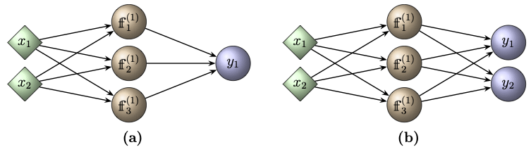
\begin{eqnarray} \boldsymbol{x}^{(l)} &=& \mathfrak{h}^{(l)} (\boldsymbol{x}^{(l-1)};\overline{W}^{(l)})\\ &=& \underset{\overline{~~~~}}{\mathscr{A}}^{(l)}\big( \underline{𝕒}(\overline{\boldsymbol{x}}^{(l-1)};\overline{W}^{(l)})\big). \end{eqnarray}(4.5)

Figure 4.1: Schematic of single layer neural networks. (a) A real-valued neural network \({\mathscr{F}_{2,3}}:\mathbb{R}^2\rightarrow \mathbb{R}\); (b) A vector-valued network \({\mathscr{F}_{2,3}}:\mathbb{R}^2\rightarrow \mathbb{R}^2\).

Example 4.1:

Illustrations of single-layer neural networks, with scalar-valued and vector-valued outputs, are depicted in Figure 4.1(a) and Figure 4.1(b), respectively.

Let us write the explicit form of the ANN shown in Figure 4.1(a). The input layer has two features, i.e., \(n_0=2\). There are two layers with the hidden layer having \(n_1=3\) neurons. Thus, the depth of the network is 2 and the width is 3. Therefore, the ANN is the function \({\mathscr{F}_{2,3}}:\mathbb{R}^2\rightarrow \mathbb{R}\) with the trainable parameter

\[\boldsymbol{\Theta} = \big( \overline{W}^{(1)}, \overline{W}^{(2)} \big),\]

where

\[ \overline{W}^{(1)} = \left(\begin{array}{lll} b^{(1)}_1 & w^{(1)}_{11}& w^{(1)}_{12}\\ b^{(1)}_2 & w^{(1)}_{21}& w^{(1)}_{22}\\ b^{(1)}_3 & w^{(1)}_{31}& w^{(1)}_{32} \end{array}\right),~~ \overline{W}^{(2)} = \left(\begin{array}{llll} b^{(2)}_1 & w^{(2)}_{11}& w^{(2)}_{12}& w^{(2)}_{13} \end{array}\right). \]

Thus, the network has 13 trainable parameters.

The affine function of the first layer is

\[ \underline{𝕒}(\overline{\boldsymbol{x}}^{(0)};\overline{W}^{(1)}) = W^{(1)}\boldsymbol{x}^{(0)} + \boldsymbol{b}^{(1)}, \]

Using the notations in (4.3), we obtain

\begin{eqnarray} \underline{𝕒}(\overline{\boldsymbol{x}}^{(0)};\overline{W}^{(1)}) &=& \left(\begin{array}{ll} w^{(1)}_{11}& w^{(1)}_{12}\\ w^{(1)}_{21}& w^{(1)}_{22}\\ w^{(1)}_{31}& w^{(1)}_{32} \end{array}\right) \left(\begin{array}{l} x^{(0)}_1 \\ x^{(0)}_2 \end{array}\right) + \left(\begin{array}{l} b^{(1)}_1 \\ b^{(1)}_2 \\ b^{(1)}_3 \end{array}\right)\\ &=& \left(\begin{array}{l} w^{(1)}_{11}x^{(0)}_1 + w^{(1)}_{12}x^{(0)}_2+ b^{(1)}_1 \\ w^{(1)}_{21}x^{(0)}_1 + w^{(1)}_{22}x^{(0)}_2+ b^{(1)}_2 \\ w^{(1)}_{31}x^{(0)}_1 + w^{(1)}_{32}x^{(0)}_2+ b^{(1)}_3 \end{array}\right). \end{eqnarray}(4.6)

The activation \(\boldsymbol{x}^{(1)}\) of the hidden layer is now obtained by applying the activation function \(\mathscr{A}^{(1)}\) of the first hidden layer on the above vector coordinatewise to get

\begin{eqnarray} \boldsymbol{x}^{(1)} &=& \underset{\overline{~~~~}}{\mathscr{A}}^{(1)}\left(W^{(1)}\boldsymbol{x}^{(0)} + \boldsymbol{b}^{(1)}\right)\\ &=&\left(\begin{array}{c} \mathscr{A}^{(1)}\big( w^{(1)}_{11}x^{(0)}_1 + w^{(1)}_{12}x^{(0)}_2 + b^{(1)}_1 \big)\\ \mathscr{A}^{(1)}\big( w^{(1)}_{21}x^{(0)}_1 + w^{(1)}_{22}x^{(0)}_2 + b^{(1)}_2 \big)\\ \mathscr{A}^{(1)}\big( w^{(1)}_{31}x^{(0)}_1 + w^{(1)}_{32}x^{(0)}_2 + b^{(1)}_3 \big) \end{array}\right). \end{eqnarray}(4.7)

Taking \(\boldsymbol{x}^{(1)}\) as the input, the output is then computed at the output layer as

\[ y = \mathscr{A}^{(2)} \big( w^{(2)}_{11} x^{(1)}_{1} + w^{(2)}_{12} x^{(1)}_{2} + w^{(2)}_{13} x^{(1)}_{3} + b^{(2)}_1 \big). \]

Observe that the right hand side of the above expression is the ANN \({\mathscr{F}_{2,3}}(\cdot\,;\boldsymbol{\Theta})\) of the network depicted in Figure 4.1(a) given by (4.1), and its explicit expression is given by

\begin{eqnarray} {\mathscr{F}_{2,3}}(\boldsymbol{x}^{(0)};\boldsymbol{\Theta}) = \mathscr{A}^{(2)}\Big( w^{(2)}_{11}\mathscr{A}^{(1)}\big( w^{(1)}_{11}x^{(0)}_1 + w^{(1)}_{12}x^{(0)}_2 + b^{(1)}_1 \big)\\ + w^{(2)}_{12}\mathscr{A}^{(1)}\big( w^{(1)}_{21}x^{(0)}_1 + w^{(1)}_{22}x^{(0)}_2 + b^{(1)}_2 \big)\\ + w^{(2)}_{13} \mathscr{A}^{(1)}\big( w^{(1)}_{31}x^{(0)}_1 + w^{(1)}_{32}x^{(0)}_2 + b^{(1)}_3 \big) + b^{(2)}_1 \Big), \end{eqnarray}(4.8)

for every input vector \( \boldsymbol{x}^{(0)}\in \mathbb{R}^{2}\).

Problem 4.1:

Derive the explicit expression for the ANN \({\mathscr{F}_{2,3}}(\boldsymbol{x}^{(0)};\boldsymbol{\Theta})\) of the network depicted in Figure 4.1(b) and give all the trainable parameters of this network.

4.1.2 Forward Propagation

The shallow network computations described in the previous subsection can be generalized to neural networks of arbitrary depth.

For fixed parameters \(\boldsymbol{\Theta}\), the network function \({\mathscr{F}_{L,\hat{n}}}:\mathbb{R}^{n_0}\rightarrow \mathbb{R}^{n_L}\) is well-defined. For every input vector \(\boldsymbol{x}\in\mathbb{R}^{n_0}\), the final output \(\boldsymbol{y}={\mathscr{F}_{L,\hat{n}}}(\boldsymbol{x}; \boldsymbol{\Theta})\) is evaluated recursively by taking the output of the \((l-1)^{\rm st}\) layer as the input to the \(l^{\rm th}\) layer, and computing

\[ \boldsymbol{x}^{(l)} = \mathfrak{h}^{(l)} \big( \boldsymbol{x}^{(l-1)};\overline{W}^{(l)} \big),~l = 1,2,\ldots, L, \]

where \(\boldsymbol{x}^{(l)}\) is called the activation of the \(l^{\rm th}\) layer. This recursive evaluation procedure is referred to as the forward propagation of the activations.

4.1.2.1 The Batch Form

Given a dataset

\[\mathcal{D} = \big\{(\boldsymbol{x}_k, \boldsymbol{y}_{k}) \mid k=1,2,\ldots, N\big\}\subset \mathbb{R}^{n_0}\times \mathbb{R}^{n_L},\]

arrange the input vectors in the \(n_0\times N\) matrix form as

\[ {A}^{(0)}:= [ \boldsymbol{x}_1~\boldsymbol{x}_2~\cdots~\boldsymbol{x}_N] = \left(\begin{array}{lllcl} x^{(0)}_{11}&x^{(0)}_{12}&\cdots&x^{(0)}_{1N}\\ x^{(0)}_{21}&x^{(0)}_{22}&\cdots&x^{(0)}_{2N}\\ \ldots &\cdots &\cdots & \cdots \\ \ldots &\cdots &\cdots & \cdots \\ x^{(0)}_{n_01}&x^{(0)}_{n_02}&\cdots&x^{(0)}_{n_0N}\\ \end{array}\right), \]

where each column corresponds to one sample.

To gain computational efficiency, it is preferable to perform forward propagation on the entire dataset in matrix form, rather than evaluating the ANN separately for each input vector.

Then the affine function takes the form

\[ \underline{𝕒}(\overline{A}^{(0)}; \overline{W}^{(1)}) = \overline{W}^{(1)}\overline{A}^{(0)}, \]

where \(\overline{A}^{(0)}\) is the augmented input matrix, the affine function is applied columnwise, and the right hand side is a \(n_1\times N\) matrix. For notational convenience, we write

\[ Z^{(l)} := \overline{W}^{(l)}\overline{A}^{(l-1)},~~l=1,2,\ldots, L. \]

and call this matrix as the pre-activation matrix of the \(l^{\rm th}\) layer.

Apply the activation function \(\underset{\overline{~~~~}}{\mathscr{A}}^{(1)}\) to get the activation matrix of the first layer as

\[ A^{(1)} =\underset{\overline{~~~~}}{\mathscr{A}}^{(1)}\big(Z^{(1)}\big). \]

Taking the activation \(A^{(1)}\) of the first layer as the input to the second layer, the activation of the second layer is computed using the formula

\[ A^{(2)} =\underset{\overline{~~~~}}{\mathscr{A}}^{(2)}\big({Z}^{(2)}\big). \]

Proceed recursively as

\[ A^{(l)} = \underset{\overline{~~~~}}{\mathscr{A}}^{(l)}\big({Z}^{(l)}\big), \quad l=1,2,\ldots,L-1, \]

for all the hidden layers.

Remark 4.2 (Activation at the Output Layer):

The choice of the activation functions at the output layer depends on the purpose of the neural network. If the network is used for regression or function approximation, then the activation function at each neuron of the output layer is the identity map and hence \(\underset{\overline{~~~~}}{\mathscr{A}}^{(L)}\) denotes the componentwise identity activation.

On the other hand, if the neural network has a multi-class classification, then the activation function at the output layer is a softmax function \(\texttt{sm}\) introduced in Subsection 1.3.6. In this case, the notation \(\underset{\overline{~~~~}}{\mathscr{A}}^{(L)}\) should not be taken as an activation function applied componentwise, rather it is a vector valued softmax function.

The following algorithm gives the computational procedure of the batch forward propagation:

Algorithm 4.1 (Batch Forward Propagation):

Input:

Given the trainable parameters
\[\boldsymbol{\Theta} = \big( \overline{W}^{(1)}, \overline{W}^{(2)}, \cdots, \overline{W}^{(L)} \big)\]
Given the dataset in the form of a \(n_0\times N\) matrix \( A^{(0)}. \)

Processing:
For each layer \(l=1,2,\ldots, L\), perform the following computation:

Augment the activation \(A^{(l-1)}\) matrix to obtain \(\overline{A}^{(l-1)}\).
Perform the matrix multiplication
\[ Z^{(l)} = \overline{W}^{(l)}\,\overline{A}^{(l-1)} \]
Apply the activation function to each element of the matrix \(Z^{(l)}\) as follows:
For \(i=1,2,\ldots, n_l\)
\(~~~~~~\)For \(j=1, 2, \ldots, N\)
\(~~~~~~~~~~~~A^{(l)}_{ij} = \mathscr{A}^{(l)}(Z^{(l)}_{ij}).\)

Output: \(Y = A^{(L)},\) which is a \(n_L\times N\) matrix

Note:

The above algorithm is written for the case where the activation of the output layer is applied componentwise. If the output layer uses the softmax function, then the activation of the output layer should be replaced by the vector-valued activation of the above remark, applied to each column of \(Z^{(L)}\).

A visualization of the above algorithm is shown in Figure 4.2

Figure 4.2: Visualization of batch forward propagation in a feedforward neural network, showing how the input passes through hidden layers to generate the final output.

Remark 4.3:

An artificial neural network can be completely specified by the tuple

\[ \big( \boldsymbol{\Theta}, \underset{\overline{~~~~}}{\mathscr{A}} \big) := \Big((\overline{W}^{(1)}, \underset{\overline{~~~~}}{\mathscr{A}}^{(1)}_{n_1}), (\overline{W}^{(2)}, \underset{\overline{~~~~}}{\mathscr{A}}^{(2)}_{n_2}),\ldots, (\overline{W}^{(L)}, \underset{\overline{~~~~}}{\mathscr{A}}^{(L)}_{n_L})\Big), \]

where \(\underset{\overline{~~~~}}{\mathscr{A}}^{(l)}_{n_l}\) denotes the activation function of the \(l^{\rm th}\) layer with the indication of the width of the layer as the suffix.

Note:

The augmented form used in Algorithm 4.1 is only for a notational convenience in the theoretical discussions. It is not the form used by the deep learning libraries such as TensorFlow and PyTorch. These libraries keep the bias separate from the weight matrix rather than augmenting.

Code 4.1 (TensorFlow and PyTorch Implementations):

\(~\)

Understand the following Python code implementing the above forward propagation algorithm
BatchForwardPropagationDirectImplementation
Understand the following Python code that implements forward propagation using TensorFlow-Keras
BatchForwardPropagationTensorFlow-Keras
In the TensorFlow-Keras implementation of a feedforward neural network, the weights, biases, and batch input \(A^{(0)}\) are handled differently from the augmented matrix format used in the theoretical formulation.
1. Describe how Keras stores the weight matrices and bias vectors for each layer, and compare this with the augmented weight matrix format \(\overline{W}^{(l)}\) we used in theory.
2. Explain the difference between the batch input format of \(A^{(0)}\) in Keras (i.e., NumPy/TensorFlow arrays) and the format we used in the theoretical framework (column-wise arrangement of samples) as well as in the first code above.
Understand the following Python code that implements forward propagation using PyTorch
BatchForwardPropagationPyTorch
State the shape of the weight and bias attributes of PyTorch. Determine whether the stored weight array agrees with \(W^{(l)}\) or with its transpose, and compare your answer with the Keras case of Question 3.

Observe that, at each layer, Algorithm 4.1 generates two matrices, namely, the pre-activation matrix \(Z^{(l)}\) and the activation matrix \(A^{(l)}\). Only the last activation \(A^{(L)}\) is required for evaluating the value of the network function. However, the matrices \(Z^{(l)}\) and \(A^{(l)}\), \(l=1,2,\ldots,L\), are needed for the evaluation of the gradient of the cost function, as we see in the next section. For this reason, the intermediate quantities computed in the forward propagation algorithm have to be retained in memory.

4.2 Backpropagation

Training a neural network amounts to minimizing a cost function \(\mathcal{C}(\boldsymbol{\Theta})\), defined over the space of all trainable parameters \(\boldsymbol{\Theta}\). In order to proceed towards the minimum faster, we need to determine the direction in the parameter space along which \(\mathcal{C}\) decreases most rapidly. This direction is given by the gradient of \(\mathcal{C}\) with respect to the weights and the biases. Backpropagation provides us with an efficient method to compute these gradients using the chain rule.

For a single neuron with the bias \(b\) and the weight vector \(\boldsymbol{w} = (w_1, w_2, \ldots, w_n)\), the gradient of a cost function \(\mathcal{C}\) is given by

\[ \nabla \mathcal{C} = \left(\frac{\partial \mathcal{C}}{\partial b}, \nabla_{\boldsymbol{w}} \mathcal{C} \right) =\left(\frac{\partial \mathcal{C}}{\partial b},~\left(\frac{\partial \mathcal{C}}{\partial w_1}, \frac{\partial \mathcal{C}}{\partial w_2}, \ldots, \frac{\partial \mathcal{C}}{\partial w_n}\right)~\right). \]

4.2.1 Gradient Computation

In this subsection, we discuss the application of the chain rule to compute the gradient of a cost function. To keep the discussions clear, we first introduce the procedure for a single neuron and then extend it to shallow networks. The extention to a general network is taken up in Subsection 4.2.2.

4.2.1.1 Gradient Computation for Neurons

Let us first consider a single neuron with the neuron function \(\text{𝕗}\). Then the output is given by \(\tilde{y} = \text{𝕗}(\boldsymbol{x};\overline{\boldsymbol{w}}) = \mathscr{A}\circ \text{𝕒}(\overline{\boldsymbol{x}};\overline{\boldsymbol{w}})\). Since \(\mathcal{C}\) measures the proximity between the true label \(y\) and the model predicted value \(\tilde{y}\), it depends on the weights and the bias only through the affine function \(\text{𝕒}\). Therefore, we have

\[ \frac{\partial \mathcal{C}}{\partial b} = \frac{\partial \mathcal{C}}{\partial \text{𝕒}} \frac{\partial \text{𝕒}}{\partial b} = \delta ~~\text{and}~~ \frac{\partial \mathcal{C}}{\partial w_k} = \frac{\partial \mathcal{C}}{\partial \text{𝕒}} \frac{\partial \text{𝕒}}{\partial w_k} = \delta\, x_k,~k=1,2,\ldots, n, \]

where

\[\delta = \frac{\partial \mathcal{C}}{\partial \text{𝕒}} = \mathcal{C}'(\tilde{y})\, \mathscr{A}'(\text{𝕒}). \]

Recall, we have computed the gradient of the cross-ratio loss function in Subsection 3.2.2

4.2.1.2 Propagation for Shallow Networks

We now discuss the gradient of the cost function associated with a single hidden layer neural network. Since the cost function depends on the trainable parameters only through the model predicted output vector \(\tilde{\boldsymbol{y}} = \boldsymbol{x}^{(2)}\) (here we have taken \(L=2\)), we have to start the gradient calculation from the output layer and progress towards the first hidden layer by applying the chain rule backwards through the layers to obtain all the required derivatives. This procedure is known as backpropagation.

Layer \(l=2\):
Following the gradient calculation at the neuron level given above, for the \(i^{\rm th}\) neuron of the output layer \(l=2\), we have

\[ \frac{\partial \mathcal{C}}{\partial b^{(2)}_i} = \delta^{(2)}_i,~~ \frac{\partial \mathcal{C}}{\partial w^{(2)}_{ij}} = \delta^{(2)}_i x^{(1)}_j, ~~i=1,2,\ldots, n_2,~j=1,2,\ldots,n_1, \]

where

\[ \delta^{(2)}_i = \frac{\partial \mathcal{C}}{\partial \text{𝕒}^{(2)}_i} ~~\text{with}~~ \text{𝕒}^{(2)}_i = \big\langle \overline{\boldsymbol{w}}^{(2)}_{i}, \overline{\boldsymbol{x}}^{(1)}\big\rangle. \]

Layer \(l=1\):
Now for the \(i^{\rm th}\) neuron of the layer \(l=1\), we have

\[ \frac{\partial \mathcal{C}}{\partial b^{(1)}_i} = \delta^{(1)}_i,~~ \frac{\partial \mathcal{C}}{\partial w^{(1)}_{ij}} = \delta^{(1)}_i x^{(0)}_j, ~~i=1,2,\ldots, n_1,~j=1,2,\ldots,n_0, \]

where

\[ \delta^{(1)}_i = \frac{\partial \mathcal{C}}{\partial \text{𝕒}^{(1)}_i} ~~\text{with}~~ \text{𝕒}^{(1)}_i(\overline{\boldsymbol{x}}^{(0)}) = \big\langle \overline{\boldsymbol{w}}^{(1)}_{i}, \overline{\boldsymbol{x}}^{(0)}\big\rangle. \]

Observe that to obtain the gradient of \(\mathcal{C}\), we only need to calculate the \(\delta\)'s, which are given layerwise.

Delta Calculation:
We still have to obtain the formulae for the \(\delta\)'s that involve the derivatives of the activation functions, just as we obtained for a single neuron above. We get these by noting that \(\text{𝕒}^{(1)}_i\) affects \(\mathcal{C}\) through \(\text{𝕒}^{(2)}\). Therefore, we write

\begin{eqnarray} \delta^{(1)}_i &=& \frac{\partial \mathcal{C}}{\partial \text{𝕒}^{(1)}_i}\\ &=& \sum_{j=1}^{n_2}\frac{\partial \mathcal{C}}{\partial \text{𝕒}^{(2)}_j}\frac{\partial \text{𝕒}^{(2)}_j}{\partial \text{𝕒}^{(1)}_i}\\ &=&\sum_{j=1}^{n_2}\delta^{(2)}_j \frac{\partial }{\partial \text{𝕒}^{(1)}_i} \big\langle \overline{\boldsymbol{w}}^{(2)}_{j}, \overline{\boldsymbol{x}}^{(1)}\big\rangle\\ &=&\sum_{j=1}^{n_2} \delta^{(2)}_j \frac{\partial }{\partial \text{𝕒}^{(1)}_i} \left(\sum_{k=1}^{n_1}w^{(2)}_{jk} \mathscr{A}^{(1)}(\text{𝕒}^{(1)}_k) + b^{(2)}_{j}\right)\\ &=&\sum_{j=1}^{n_2} \delta^{(2)}_j w^{(2)}_{ji}\mathscr{A}^{(1)'}(\text{𝕒}^{(1)}_i)\\ &=&\mathscr{A}^{(1)'}(\text{𝕒}^{(1)}_i)\sum_{j=1}^{n_2} \delta^{(2)}_j w^{(2)}_{ji}. \end{eqnarray}(4.9)

Problem 4.2:

Consider an ANN with \(L=2\) with the logistic activation function and the binary cross-entropy cost function

\[ \mathcal{C}(\boldsymbol{y}, \tilde{\boldsymbol{y}}) = -\sum_{k=1}^{n_L} y_k \ln \tilde{y}_k - \sum_{k=1}^{n_L} (1-y_k) \ln (1-\tilde{y}_k). \]

Find the expression for \(\delta_i^{(1)}\).

4.2.2 The Backpropagation Algorithm

In the previous subsection, we have discussed how the chain rule is used in the backpropagation process to calculate the gradients of the cost function \(\mathcal{C}\) with respect to the trainable parameters. In this subsection, we discuss the backpropagation algorithm to compute the gradients of a given cost function \(\mathcal{C}\) in all the layers of a general feedforward network of depth \(L\).

Algorithm 4.2 (Backpropagation Algorithm):

Input:

Choose an input vector \(\boldsymbol{x}\) and its corresponding true label vector \(\boldsymbol{y}\).
Choose values for the trainable parameters in \(\boldsymbol{\Theta}\).

Processing:

Perform the forward propagation to obtain the activations as follows:
Forward propagation: For \(l=1,2,\ldots, L\), compute
\[ x^{(l)}_j = \mathscr{A}^{(l)}\left( \sum_{k=1}^{n_{l-1}} w_{jk}^{(l)} x_{k}^{(l-1)} + b_{j}^{(l)}\right),~j=1,2,\ldots, n_l, \]
and take the model predicted output as \(\tilde{\boldsymbol{y}} = \boldsymbol{x}^{(L)}\).
Calculate the \(\delta\)'s at the output layer \(L\) using the following formula:
\begin{eqnarray} \delta^{(L)}_j &=& \frac{\partial \mathcal{C}}{\partial \text{𝕒}^{(L)}_j}(\boldsymbol{y}, \tilde{\boldsymbol{y}})\\ &=& \frac{\partial \mathcal{C}}{\partial x^{(L)}_j}(\boldsymbol{y}, \tilde{\boldsymbol{y}})\,\mathscr{A}^{(L)'}(\text{𝕒}^{(L)}_j),~~j=1,2,\ldots, n_L, \end{eqnarray}(4.10)
where \(\text{𝕒}^{(L)}_j=\big\langle \overline{\boldsymbol{w}}^{(L)}_j, \overline{\boldsymbol{x}}^{(L-1)}\big\rangle.\)
Next perform the backpropagation for calculating the deltas in each hidden layer using the following formula:
Backpropagation for deltas: For \(l=L-1,L-2,\ldots, 1\), compute
\begin{eqnarray} \delta^{(l)}_i &=& \mathscr{A}^{(l)'}(\text{𝕒}^{(l)}_i)\sum_{j=1}^{n_{l+1}} \delta^{(l+1)}_j w^{(l+1)}_{ji},~~i=1,2,\ldots, n_l. \end{eqnarray}(4.11)
Compute the components of the gradient of \(\mathcal{C}\) as follows:
For \(l=L,L-1,\ldots, 1\),
\[ \frac{\partial \mathcal{C}}{\partial b^{(l)}_i} = \delta^{(l)}_i,~~ \frac{\partial \mathcal{C}}{\partial w^{(l)}_{ij}} = \delta^{(l)}_i x^{(l-1)}_j, ~~i=1,2,\ldots,n_{l},~ j=1,2,\ldots,n_{l-1}, \]

Output: All the gradient components

\[\nabla_{\boldsymbol{\Theta}} \mathcal{C} =\Big( \big(\nabla_{\boldsymbol{b}^{(l)}} \mathcal{C}, \nabla_{W^{(l)}}\mathcal{C}\big) \Big)_{l=1}^L.\]

Note:

PyTorch and TensorFlow use reverse-mode automatic differentiation, which is an efficient way of implementing the backpropagation. We omit the details in this course. Interested readers can refer to Bishop and Bishop (2024), section 8.2 on page 244 for the details on this approach.

4.2.3 Batch Form, Computational Cost, and Gradient Checking

Algorithm 4.2 computes the gradient of a cost function with respect to the trainable parameters for a single input vector \(\boldsymbol{x}\). For computational efficiency, we need the gradient to be computed for a batch of inputs, where the computation is performed in the matrix form introduced in Section 4.1.

It is convenient to separate the comparison of one prediction with one label from the aggregation of these comparisons over the dataset.

Definition 4.1 (Loss Function and Cost Function):

A loss function is a function

\[ \ell: \mathbb{R}^{n_L}\times \mathbb{R}^{n_L} \rightarrow [0,\infty), \]

where \(\ell(\boldsymbol{y}, \tilde{\boldsymbol{y}})\) measures the discrepancy between a label \(\boldsymbol{y}\) and the corresponding prediction \(\tilde{\boldsymbol{y}}\). Given a dataset \(\mathcal{D}\) with \(N\) samples, the associated cost function is the average

\begin{eqnarray} \mathcal{C}(\boldsymbol{\Theta}) = \frac{1}{N} \sum_{k=1}^{N} \mathcal{C}_k(\boldsymbol{\Theta}), \end{eqnarray}(4.12)

where \( \mathcal{C}_k(\boldsymbol{\Theta}) := \ell\big(\boldsymbol{y}_k, \tilde{\boldsymbol{y}}_k\big) \) is called the per-sample cost.

Recall from Section 4.1 that \(A^{(L)}\) is the activation matrix of the output layer whose \(k^{\rm th}\) column is the network prediction \(\tilde{\boldsymbol{y}}_k\) of the true label \(\tilde{\boldsymbol{y}}_k\). We write the labels of the dataset as the \(n_L\times N\) matrix

\[ Y := [\,\boldsymbol{y}_1~\boldsymbol{y}_2~\cdots~\boldsymbol{y}_N\,], \]

so that the \(k^{\rm th}\) column of \(Y\) is the label of the \(k^{\rm th}\) sample.

Similarly, for \(l=1,2,\ldots, L\), we write the \(n_l\times N\) activation matrix \(A^{(l)}\) of the \(l^{\rm th}\) layer as

\[A^{(l)} = [\, \boldsymbol{x}^{(l)}_1~\boldsymbol{x}^{(l)}_2~\cdots~\boldsymbol{x}^{(l)}_N],\]

so that \(\tilde{\boldsymbol{y}} = \boldsymbol{x}^{(L)}_k\) is the prediction of the network for the \(k^{\rm th}\) sample.

Observe that the per-sample cost \(\mathcal{C}_k\) depends on the trainable parameters only through the \(k^{\rm th}\) column of the activation matrix \(A^{(L)}\) of the output layer .

4.2.3.1 The Delta Matrices

Define the \(n_l \times N\) delta matrix \(\Delta^{(l)}\) for the \(l^{\rm th}\) layer as

\begin{eqnarray} \Delta^{(l)}_{ik} := \frac{\partial \mathcal{C}_k}{\partial Z^{(l)}_{ik}}, ~~i=1,2,\ldots, n_l,~k=1,2,\ldots,N. \end{eqnarray}(4.13)

The \(k^{\rm th}\) column of \(\Delta^{(l)}\) is the vector of the quantities \(\delta^{(l)}_i\) of the previous subsection, computed for the \(k^{\rm th}\) sample. Note that the cost of the \(k^{\rm th}\) sample does not depend on the pre-activations of any other sample, and therefore the columns of \(\Delta^{(l)}\) are computed independently of each other.

4.2.3.2 Backward Recursion in Matrix Form

We first record the derivative of a coordinatewise activation function in matrix form. For a given activation function \(\mathscr{A}^{(l)}:\mathbb{R}\rightarrow \mathbb{R}\) and a matrix \(Z\) of size \(n_l\times N\), we use the notation \(\underset{\overline{~~~~}}{\mathscr{A}}^{(l)'}(Z)\) for the \(n_l\times N\) matrix whose \((i,k)^{\rm th}\) entry is \(\mathscr{A}^{(l)'}(Z_{ik})\). We also use the notation \(\odot\) for the entrywise product, called the Hadamard product, of two matrices of the same size.

Output layer: Assume that the activation of the output layer is applied coordinatewise. Since \(\mathcal{C}_k\) depends on \(Z^{(L)}_{ik}\) only through \(A^{(L)}_{ik} = \mathscr{A}^{(L)}(Z^{(L)}_{ik})\), the chain rule gives

\[ \Delta^{(L)}_{ik} = \frac{\partial \mathcal{C}_k}{\partial A^{(L)}_{ik}}\, \mathscr{A}^{(L)'}\big(Z^{(L)}_{ik}\big), \]

which in matrix form reads

\begin{eqnarray} \Delta^{(L)} = \frac{\partial \mathcal{C}}{\partial A^{(L)}} \odot \underset{\overline{~~~~}}{\mathscr{A}}^{(L)'}\big(Z^{(L)}\big), \end{eqnarray}(4.14)

where \(\dfrac{\partial \mathcal{C}}{\partial A^{(L)}}\) denotes the \(n_L\times N\) matrix with entries \(\dfrac{\partial \mathcal{C}_k}{\partial A^{(L)}_{ik}}\).

Hidden layers: For \(l = L-1, L-2, \ldots, 1\), the pre-activation of the \((l+1)^{\rm st}\) layer is

\[ Z^{(l+1)}_{ik} = \sum_{j=1}^{n_l} W^{(l+1)}_{ij} A^{(l)}_{jk} + b^{(l+1)}_i, ~~\text{with}~~ A^{(l)}_{jk} = \mathscr{A}^{(l)}\big(Z^{(l)}_{jk}\big). \]

Hence \(Z^{(l)}_{jk}\) influences \(\mathcal{C}_k\) only through the entries \(Z^{(l+1)}_{ik}\), \(i=1,2,\ldots, n_{l+1}\), of the same column. The chain rule therefore gives

\begin{eqnarray} \Delta^{(l)}_{ik} &=& \sum_{j=1}^{n_{l+1}} \frac{\partial \mathcal{C}_k}{\partial Z^{(l+1)}_{jk}} \frac{\partial Z^{(l+1)}_{jk}}{\partial Z^{(l)}_{ik}}\\ &=& \left(\sum_{j=1}^{n_{l+1}} W^{(l+1)}_{ji}\,\Delta^{(l+1)}_{jk} \right) \mathscr{A}^{(l)'}\big(Z^{(l)}_{ik}\big)\\ &=& \Big[\big(W^{(l+1)}\big)^\top \Delta^{(l+1)}\Big]_{ik}\, \mathscr{A}^{(l)'}\big(Z^{(l)}_{ik}\big), \end{eqnarray}(4.15)

that is,

\begin{eqnarray} \Delta^{(l)} = \Big[\big(W^{(l+1)}\big)^\top \Delta^{(l+1)}\Big] \odot \underset{\overline{~~~~}}{\mathscr{A}}^{(l)'}\big(Z^{(l)}\big), ~~l=L-1, L-2,\ldots, 1. \end{eqnarray}(4.16)

Note:

Observe that the matrix appearing in (4.16) is the weight matrix \(W^{(l+1)}\) and not the augmented weight matrix \(\overline{W}^{(l+1)}\). The bias does not depend on the activation of the previous layer, and therefore the first column of \(\overline{W}^{(l+1)}\) has to be removed before transposing.

Cost Gradients: Since \(Z^{(l)}_{ik} = \sum_{j} \overline{W}^{(l)}_{ij}\,\overline{A}^{(l-1)}_{jk}\), we have

\[ \frac{\partial \mathcal{C}}{\partial \overline{W}^{(l)}_{ij}} = \frac{1}{N}\sum_{k=1}^{N} \frac{\partial \mathcal{C}_k}{\partial Z^{(l)}_{ik}}\, \overline{A}^{(l-1)}_{jk} = \frac{1}{N}\Big[\Delta^{(l)}\big(\overline{A}^{(l-1)}\big)^\top\Big]_{ij}, \]

and therefore

\begin{eqnarray} \frac{\partial \mathcal{C}}{\partial \overline{W}^{(l)}} = \frac{1}{N}\, \Delta^{(l)}\big(\overline{A}^{(l-1)}\big)^\top, ~~l=1,2,\ldots, L, \end{eqnarray}(4.17)

which is a matrix of size \(n_l\times (n_{l-1}+1)\), of the same size as \(\overline{W}^{(l)}\). Since the first row of \(\overline{A}^{(l-1)}\) consists of ones, the first column of (4.17) is

\[ \frac{\partial \mathcal{C}}{\partial \boldsymbol{b}^{(l)}} = \frac{1}{N}\, \Delta^{(l)} \mathbf{1}_N, \]

where \(\mathbf{1}_N\in \mathbb{R}^N\) is the column vector of ones, and the remaining columns give the derivatives with respect to \(W^{(l)}\). Thus, the augmented form (4.17) gives the derivatives of the cost function with respect to the weights and the bias in a single matrix product.

The above computations are collected in the following backpropagation algorithm applicable for a network whose output activation is applied coordinatewise.

Algorithm 4.3 (Batch Backpropagation):

Input:

The trainable parameters \(\boldsymbol{\Theta} = \big( \overline{W}^{(1)}, \overline{W}^{(2)}, \cdots, \overline{W}^{(L)} \big)\).
The input matrix \(A^{(0)}\) of size \(n_0\times N\) and the label matrix \(Y\) of size \(n_L\times N\).

Processing:

Run Algorithm 4.1 and retain the matrices \(Z^{(l)}\), \(l=1,2,\ldots,L\), and \(A^{(l)}\), \(l=0,1,\ldots,L\).
Compute the delta matrix of the output layer using (4.14).
For \(l=L-1, L-2, \ldots, 1\), compute
\[ \Delta^{(l)} = \Big[\big(W^{(l+1)}\big)^\top \Delta^{(l+1)}\Big] \odot \underset{\overline{~~~~}}{\mathscr{A}}^{(l)'}\big(Z^{(l)}\big). \]
For \(l=1,2,\ldots, L\), compute
\[ \frac{\partial \mathcal{C}}{\partial \overline{W}^{(l)}} = \frac{1}{N}\, \Delta^{(l)}\big(\overline{A}^{(l-1)}\big)^\top. \]

Output: The matrices \(\dfrac{\partial \mathcal{C}}{\partial \overline{W}^{(l)}}\), \(l=1,2,\ldots, L\).