Introduction to Neurons

This chapter is mainly divided into two sections. The first Section «Click Here» presents a few motivating examples that work similarly to artificial neurons. The mathematical formulation of artificial neurons is then provided in the second Section «Click Here», and the reason behind the name neuron is made clear by comparing the formulation with the functionality of biological neurons. The chapter ends with an outline of the algorithm to learn a neuron model.

Motivating Example

In this we give two simple examples to set a fundamental idea behind the way artificial neurons are formulated. The first example is intuitive from physics that illustrates an important and commonly used activation function called rectifiable linear unit (ReLU) and another from electric circuit which involves the step function as the activation function which is fundamental in defining perceptrons.

Water Source-Sink Control Problem

Note:

Refer to Section 1.1 (page 3) in the following book:

Calin, Ovidiu, Deep Learning Architectures: A Mathematical Approach, Springer, 2020.

Click here to see the details of the book

Mathematical Problem

The task is to adjust the knobs and the rate of outlet, depending on the inlet water pressure, such that the volume of water in the tank after time \(t\) is exactly at \(V\).

The problem can be posed mathematically as follows: Given \(V>0\), \(t>0\), and the vector \(\boldsymbol{P} = (P_1, P_2, \ldots, P_n)\), for \(P_i> 0\), find a vector \(\boldsymbol{w} = (w_1, w_2, \ldots, w_n)\) and \(R>0\) such that

\[ \phi_t\big(\boldsymbol{P} \cdot \boldsymbol{w} - R\big) = V. \]

Remark:

It is easy to see that there are infinitely many solutions for this problem and it is straightforward to choose one. For instance, choose any set of values \(w_k> 0\), for each \(k=1,2,\ldots, n\), such that \(\boldsymbol{P} \cdot \boldsymbol{w} > {V}/{t}\) and then choose

\[ R = \boldsymbol{P} \cdot \boldsymbol{w} - \frac{V}{t}. \]

Note:

If each component of \(\boldsymbol{w}\) is bounded, then we may not have a solution for the above problem.

The mathematical problem posed above takes \((\boldsymbol{P},V)\in (0,\infty)^n \times (0,\infty)\) as an input and provides \((\boldsymbol{w},R)\) as an output. Often the interest is to obtain one set of parameters \((\boldsymbol{w}^*,R^*)\) such that

\[ V \approx \phi_t \left( \boldsymbol{P}\cdot \boldsymbol{w}^* - R^* \right), \]

for all \((\boldsymbol{P},V)\in \mathcal{D},\) where

\begin{eqnarray} \mathcal{D} = \big\{\big(\boldsymbol{P}^{(k)},V^{(k)}\big) ~|~k = 1,2,\dots, N\big\} \subset (0,\infty)^n\times (0,\infty), \end{eqnarray}

(1.1)

is a given finite dataset. Further, it is desirable to obtain an optimal pair \((\boldsymbol{w}^*,R^*)\) that best fits the given dataset.

Problem:

Consider the dataset \(\mathcal{D}\) with \(n=3\) and \(N=5\) as given in the following table:

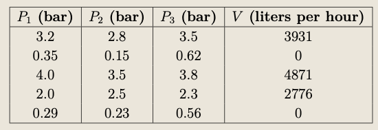
Given \(t=1\) hour and the outlet flow rate is \(R=450\) L/h, determine the weight vector \(\boldsymbol{w} = (w_1, w_2, w_3)\).

Hint:

Since \(V\) is defined using \(\phi_t\), it is enough to have a negative value for the affine function whenever \(V=0\) in the above dataset.

Electric Circuit

Note:

Refer to Section 1.2 (page 6) in the following book:

Calin, Ovidiu, Deep Learning Architectures: A Mathematical Approach, Springer, 2020.

Click here to see the details of the book

Mathematical Problem

The problem we are interested in the present example is similar to the one posed in the above example.

Given a dataset \(\mathcal{D} = \{(\boldsymbol{x}^{(k)}, y^{(k)})~|~k=1,2,\cdots, N\} \subset \mathbb{R}^n \times (0, \infty)\), the problem of interest is to find the weights vector and bias \((\boldsymbol{w}^*, \beta^*)\) such that

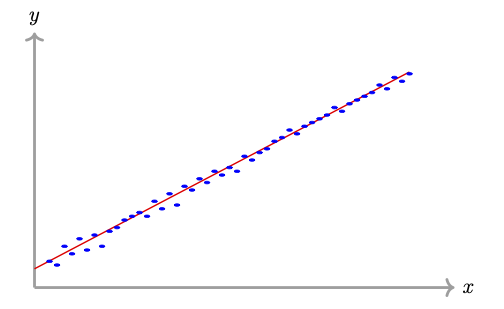
\[ y \approx c\phi_0\big(\boldsymbol{w}^{*}\cdot \boldsymbol{x} - \beta^*\big), ~~\text{for all}~(\boldsymbol{x}, \beta)\in \mathcal{D}. \]

Linear Regression

Linear regression is one of the most fundamental and widely used methods in both statistics and machine learning. It aims to model the relationship between a dependent variable and one or more independent variables by fitting a linear equation to the observed data.

In linear regression, the given dataset consists of

A set of observations for the dependent or the response variable: \( y^{(1)}, y^{(2)}, \ldots, y^{(N)} \)

Corresponding sets of observations for the independent or the predictor variables: \(\boldsymbol{x}^{(1)}, \boldsymbol{x}^{(2)}, \ldots, \boldsymbol{x}^{(N)}\) where \(\boldsymbol{x}=(x_{1}, x_{2}, \ldots, x_{n})\in \mathbb{R}^n\). The objective is to find the regression coefficients \( w_0, w_1, \ldots, w_n \) that best describe the linear relationship between the independent variables and the dependent variable. Thus, the basic form of a linear regression model is

\begin{eqnarray} y = w_0 + w_1 x_1 + w_2 x_2 + \ldots + w_n x_n + \epsilon \end{eqnarray}

(1.2)

where \( \epsilon \) is the error term, representing the deviation of the observed values from the true values.

An illustration for the case \(n=1\) is depicted in the following figure:

Illustration of a linear regression model with fitted line and data points.

Mathematical Problem

Let us give a precise formulation of a linear regression model.

For the given dataset

\begin{eqnarray} \mathcal{D} = \big\{(\boldsymbol{x}^{(k)}, y^{(k)})~|~\boldsymbol{x}^{(k)}\in \mathbb{R}^n,~ y^{(k)}\in \mathbb{R},~k=1,2,\cdots, N\}, \end{eqnarray}

(1.3)

the primary objective is to find the values of the coefficients \((w_0, w_1, \ldots, w_n)\) such that the sum of the squared errors is minimized.

In other words, we aim to minimize the sum of squares error function

\begin{eqnarray} L(\overline{\boldsymbol{w}}) = \sum_{i=1}^N \Big( y_i - (w_0 + w_1 x_{i1} + w_2 x_{i2} + \ldots + w_n x_{in}) \Big)^2, \end{eqnarray}

(1.4)

where \(\overline{\boldsymbol{w}}=(w_0, w_1, \ldots, w_m)\) is the regression coefficient vector. That is, to find the optimal coefficient \(\overline{\boldsymbol{w}}^*\) such that

\begin{eqnarray} L(\overline{\boldsymbol{w}}^*) = \min_{ \overline{\boldsymbol{w}}} L(\overline{\boldsymbol{w}}) ~~{or}~~ \overline{\boldsymbol{w}}^* = {arg} \min_{\overline{\boldsymbol{w}}} L(\overline{\boldsymbol{w}}) \end{eqnarray}

(1.5)

The optimal coefficients best fit the given dataset in the least squares sense and this method is known as the least squares method.

Artificial Neurons

The physical problems discussed in Section «Click Here» resemble the mathematical framework of an artificial neuron involving weights (control knobs and resistors), a bias term acting as a threshold (like the outflow rate and flow of current to ground), and a nonlinear activation function.

Mathematical Formulation

We now formalize the physical intuitions through the mathematical definition of an artificial neuron.

Definition:

[Artificial Neuron]

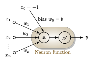
An artificial neuron is a tuple \( (\overline{\boldsymbol{w}}, \mathscr{A}) \), where

\(\overline{\boldsymbol{w}}=(w_0, \boldsymbol{w})\in \mathbb{R}\times \mathbb{R}^{n}\) is the augmented weights vector, with \(w_0=b\in \mathbb{R}\) as the bias and \(\boldsymbol{w}=(w_1,w_2,\ldots,w_n)\in \mathbb{R}^n\) as the weight vector; and
\(\mathscr{A}:\mathbb{R}\rightarrow \mathbb{R}\), is an (nonlinear) activation function.

Given an augmented input vector \(\overline{\boldsymbol{x}}=(x_0,\boldsymbol{x})\in \{-1\}\times \mathbb{R}^{n}\), with \(x_0=-1\) and \(\boldsymbol{x}=( x_1,x_2,\ldots,x_n)\in \mathbb{R}^n\) is an input vector, the output \(y\) of the neuron is defined as

\[ y = \mathscr{A}\big(\overline{\boldsymbol{w}}\cdot \overline{\boldsymbol{x}}\big). \]

For a given \(\overline{\boldsymbol{w}}\), the right hand side function is the composition of the affine function \(\text{𝕒}: \{-1\}\times \mathbb{R}^n\rightarrow \mathbb{R}\) given by

\[ \text{𝕒}(\overline{\boldsymbol{x}};\overline{\boldsymbol{w}}) = \sum_{k=0}^n w_k x_k = \sum_{k=1}^n w_k x_k - b, \]

and the activation function \(\mathscr{A}\). We define the neuron function (or the primitive function) \(\text{𝕗}:\{-1\}\times \mathbb{R}^n\rightarrow \mathbb{R}\) as

\begin{eqnarray} \text{𝕗}(\overline{\boldsymbol{x}};\overline{\boldsymbol{w}}) = \mathscr{A}(\text{𝕒}(\overline{\boldsymbol{x}};\overline{\boldsymbol{w}}) ). \end{eqnarray}

(1.6)

A schematic diagram of an artificial neuron is depicted in the following figure.

Schematic of an artificial neuron architecture.

Note:

Since the information flows from the input layer through the function evaluation to the output without any feedback, an artificial neuron can be regarded as part of a feedforward architecture.

An artificial neuron can be viewed as a special case of a single-layer neural network with just a single output unit.

Note:

See Section 5.1 (page 133) in the following book:

Calin, Ovidiu, Deep Learning Architectures: A Mathematical Approach, Springer, 2020.

Click here to see the details of the book

Note the notational differences between our definition above and the definition given in the book. For the examination point of view, students are requested to follow the notations used in our notes.

Example:

We are already familiar with two real-world examples that can be interpreted within the framework of an artificial neuron.

The water supply problem discussed in Section «Click Here» can be viewed as an artificial neuron \((\overline{\boldsymbol{w}}, \texttt{ReLU})\), where
\[ \texttt{ReLU}(x) = \max\{0, x\}, \]
and the bias \(b\) is the outflow rate \(R\).
The electric circuit problem discussed in Section «Click Here» can also be viewed as an artificial neuron \((\overline{\boldsymbol{w}}, H)\), where \(H\) denotes the Heaviside function given by
\[ H(x) = \left\{\begin{array}{lc} 0,&\text{if}~x<0\\ 1,&\text{if}~x\ge 0 \end{array}\right. \]
An artificial neuron with Heaviside function as the activation function is called the perceptron. We will discuss perceptrons in more details in Section «Click Here».

Comparison with Biological Neurons

The mathematical definition of \(\text{𝕗}\) (given in Definition «Click Here» ) is named as neuron by taking the inspiration from the biological neurons in brains. To have a clear understanding of these two concepts, we briefly understand the structure and the functionality of biological neurons in brains and then make a comparison with the artificial neuron formulation.

From the Definition «Click Here» on artificial neurons, we see that an artificial neuron includes a simple mathematical function (neuron function) with inputs, weights, bias, activation function and output. On the other hand, a biological neuron is a specialized type of cell in the nervous system with dendrites, soma, axon, and synapses. Biological neurons are responsible for transmitting and processing information through electrical and chemical signals.

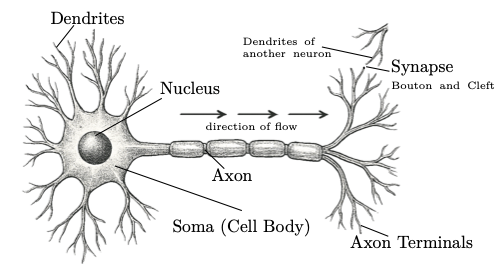
An illustration of a biological neuron. The direction of the flow of information during neurotransmission is indicated by three arrows.

A typical neuron has four main parts (shown in the above figure):

Dendrites: Branch-like structures that receive input signals from other neurons in the form of chemical signals, specifically neurotransmitters.
Soma (Cell Body): Contains the nucleus and most of the cell's organelles where input signals (electrical impulses) are integrated and a nonlinear threshold is applied. If the combined input exceeds this threshold, the axon hillock triggers an action potential, which is then propagated down the axon.
Axon: A long projection that transmits electrical signals from the soma to other neurons. The axon terminal of one neuron connects to the dendrites of another neuron via synapses.
Synaptic Boutons: These are the small, bulb-like endings of axon terminals that are involved in transmitting signals to other neurons. When an electrical signal (action potential) reaches a synaptic bouton, it triggers the release of chemical messengers called neurotransmitters into the synaptic cleft, which is a tiny gap between the axon terminal and the dendrite of the next neuron. Electrical signals cannot cross this gap directly, so neurotransmitters are used to carry the signal across.

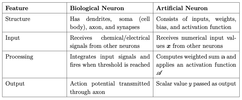
Comparison of Biological and Artificial Neurons

A comparison between biological neurons and artificial neurons is summarized in the above table. As we can see, biological neurons are more complex in nature, whereas artificial neurons are simplified mathematical models that only resemble biological neurons. Artificial neurons are not intended to be accurate models of biological neurons. Rather, they are designed to mimic certain features, such as signal integration and nonlinear activation, to build systems capable of performing tasks through self-learning, giving rise to artificial intelligence.

A neuron can connect to many other neurons through its axon terminals, and similarly, it can receive inputs from several neurons via its dendrites, forming a biological neural network. Similarly, multiple artificial neurons can be connected through layers to form an artificial neural network, which we will discuss in a later chapter.

Note:

Throughout this course, the term ‘neuron’ refers to an artificial neuron. Discussions involving biological neurons will indicate this explicitly. This convention is adopted, as the focus of the course is on artificial neural networks, and our discussions on biological neural networks are intended only for motivational purposes.

Problem:

At a party, Mrs. Sahana is offered several glasses of juice. The juices are either mango or orange, and they look quite similar. To identify mango juice, her brain subconsciously evaluates three features:

\(x_1\): Smell intensity (scale 0-10; mango juice has a stronger smell),
\(x_2\): Color richness (scale 0-10; varies between orange and yellow),
\(x_3\): Pulp density (scale 0-10; mango juice is thicker).

Model Mrs. Sahana's decision-making using an artificial neuron by indicating appropriate parameters and the activation function, but describe its working using the terminology of biological neurons as follows:

The sensory inputs arrive at the neuron's dendrites.
Each input is modulated by a corresponding synaptic weight.
These weighted signals are summed in the cell body and combined with a bias, representing the neuron's threshold.
If the total input exceeds a threshold (modeled by an activation function), the neuron fires an action potential.

Choose some values for the synaptic weights (as per your choice) and the bias, and specify a step activation function. Then, provide two specific sets of input values \((x_1,x_2,x_3)\): one for which the neuron classifies the juice as {orange}, and another for which it classifies the juice as {mango}.

Supervised Learning: An Overview

The mathematical formulation of a neuron (AN) takes \(\boldsymbol{x}=(x_1,x_2\ldots,x_n)\in \mathbb{R}^{n}\) as input and computes the output \(y\in \mathbb{R}\) as the value of the neuron function \(\text{𝕗}\). A complete AN model for a given problem therefore involves a well-defined neuron function, which in turn includes three choices, namely,

the dimension of the input vector \(n\);
a suitably chosen activation function \(\mathscr{A}\); and
a fixed choice of the bias and weights \(\overline{\boldsymbol{w}}=(b,\boldsymbol{w})\in \mathbb{R}\times \mathbb{R}^{n}\).

The choice of \(n\) and \(\mathscr{A}\) depends on the problem under consideration. Whereas, the choice of \(\overline{\boldsymbol{w}}\) is more mathematical and is achieved through some optimization method.

The process of obtaining \(\overline{\boldsymbol{w}}=(b, \boldsymbol{w})\) is referred to as learning a model (or training a model) from a given dataset \(\mathcal{D} \subset \mathbb{R}^{n} \times \mathbb{R}\) of the form

\[ \mathcal{D} = \{ (\boldsymbol{x}_k, y_k)~|~k=1,2,\ldots, N\}, \]

where \(\boldsymbol{x}_k\in \mathbb{R}^n\) is an input vector (also called a feature vector) and \(y_k \in \mathbb{R}\) is the corresponding output or label. The dataset \(\mathcal{D}\) is called a labeled dataset, and each point \((\boldsymbol{x}_k, y_k)\) in \(\mathcal{D}\) is called an example or a training sample.

Learning from such a labeled dataset is called supervised learning, where the goal is to approximate a function (or a model) that maps inputs \(\boldsymbol{x}_k\) to outputs \(y_k\).

A general outline of the learning procedure is as follows:

Data Preparation: As a first step, we decompose the dataset \(\mathcal{D}\) into three disjoint sets,

\begin{eqnarray} \mathcal{D} = \mathcal{D}_\text{train} \cup \mathcal{D}_\text{val} \cup \mathcal{D}_\text{test}. \end{eqnarray}

(1.7)

Here, \(\mathcal{D}_\text{train}\) is the training set, \(\mathcal{D}_\text{test}\) is the test set, and \(\mathcal{D}_\text{val}\) is the valudation set. Typically, \(\mathcal{D}_\text{train}\) contains a significantly larger portion of the data, often at least 70% of \(\mathcal{D}\), selected randomly in an unbiased manner. Let us use the notation

\[ \mathcal{D}_\text{train} := \big\{(\boldsymbol{x}_{k}^\text{train},y_{k}^\text{train}) ~|~k = 1,2,\dots, N_\text{train}\big\}, \]

where \(N_\text{train} = \#(\mathcal{D}_\text{train})\).

Training a Model: Consider a suitable cost function (error) \(C(b, \boldsymbol{w})\) defined on the training dataset \(\mathcal{D}_\text{train}\). The goal is to find parameters \((b, \boldsymbol{w})\) that minimize the cost function, i.e.,

\[ (b^*, \boldsymbol{w}^*) = \text{argmin}_{b, { \boldsymbol{w}}} C(b, \boldsymbol{w}). \]

For instance, a commonly used cost function is the mean squared error

\begin{eqnarray} C(b, \boldsymbol{w}) = \frac{1}{N_\text{train}} \sum_{k=1}^{N_\text{train}} \big( \mathscr{A}(\boldsymbol{w} \cdot \boldsymbol{x}_{k}^\text{train} - b) - y_{k}^\text{train} \big)^2, \end{eqnarray}

(1.8)

where \(\mathscr{A}\) is the activation function of the neuron.

An optimization method such as the gradient descent method is used to compute \( (b^*, \boldsymbol{w}^*) \). This step is called the training step or learning step.

Once the optimal parameters are computed by minimizing the cost on the training data, we typically say that the model is trained.

Evaluating the Model: The next step is to assess how well the trained model performs on unseen data. For this, we compute the cost function on the test dataset \(\mathcal{D}_\text{test}\). If this value is sufficiently small, we say that the model `generalizes well' to unseen data. This step is called testing step. If the model does not generalize well, then we need to apply additional techniques to improve generalization, such as regularization, or early stopping, or collecting more data, or architecture changes.

Regularization generally includes fine tuning some key parameters, referred to as hyperparameters. The validation set \(\mathcal{D}_\text{val}\) is used to tune hyperparameters.