Training Neural Networks

An artificial neural network (ANN) consists of several parameters, which can be broadly categorized into two types, namely, trainable (or learnable) parameters and hyperparameters. Training a neural network is the process of determining appropriate values of the trainable parameters (weights and biases) such that the ANN function (see the Definition«Click Here») approximates the required input-output mapping. Often, such mappings are implicitly represented in a training data and the trainable parameters of the network are iteratively updated to minimize the error between the predicted outputs and the true outputs. The error is quantified by an appropriately chosen loss function, and when averaged over the entire dataset, it is referred to as a cost function.

The minimization of a cost function depends on the knowledge of how the changes in the network parameters affect the cost. This requires the computation of the gradient of the cost function with respect to the parameters. The backpropagation algorithm can be used to efficiently compute these gradients by propagating errors backward through the network, starting from the output layer to the first hidden layer. Once gradients are available, the parameters are updated using optimization algorithms. The most basic method is the gradient descent method, where parameters are iteratively updated in the direction opposite to the gradient in order to reduce the cost. We also have some important variants of this method, such as the stochastic gradient descent (SGD) method and the SGD method with momentum (SGDM) to improve training efficiency and stability.

In Section «Click Here», we list some commonly used cost functions. The backpropagation algorithm and the gradient descent methods are then discussed in Section «Click Here».

Cost Functions

The choice of cost function is fundamental to the training of neural networks. Since the optimization methods that we consider rely on the computation of gradients of the cost function, it is generally preferable to use sufficiently smooth cost functions. Among the most widely used cost functions are the mean square error (MSE) and the cross-entropy function (see Remark«Click Here»). In this section, we define these cost functions along with a few other commonly used alternatives.

Before defining the cost functions, we first fix the notations.

For given input and output dimensions \(n_0, n_L\in \mathbb{N}\), we consider a dataset

For a given depth \(L\in \mathbb{N}\), and the network dimensions \(n_0, n_1, \ldots, n_L\in \mathbb{N}\) with the width \(\hat{n}=\max\{n_1, \ldots, n_{L-1}\}\), the predicted output of the ANN

for an input \(\boldsymbol{x}_k\) is denoted by

where \({\mathscr{F}_{L,\hat{n}}}\) is given in the Definition«Click Here».

The aim is to consider an appropriate cost function \(\mathcal{C}(\boldsymbol{\Theta})\) and look for the trainable parameters \(\boldsymbol{\Theta}^*\) such that

In the following subsections, we define some of the commonly used cost functions.

Mean Square Error

The mean square error (MSE) function is defined as

where \((X,Y)\) are random variables representing the input and output, \( \tilde{Y}={\mathscr{F}_{L,\hat{n}}}(X; \boldsymbol{\Theta})\) is the ANN predictor of \(Y\) corresponding to the input \(X\), and \(\mathbb{E}\) denotes expectation with respect to the underlying data distribution.

Often the true probability distribution of the data is unknown and therefore, the empirical mean square error is considered as an approximation, which is given by

Cross-Entropy

Recall that while discussing a suitable cost function for learning the logistic regression model (see Remark«Click Here»), we derived it from the negative log-likelihood. We then observed that minimizing the negative log-likelihood is equivalent to minimizing cross-entropy. This choice is natural because the true labels \(y\) come from some unknown distribution \(p(y|x)\), whereas the model predicts \(\hat{p}(y|x; \boldsymbol{\Theta})\). Since, we want our model distribution \(\hat{p}\) to be as close as possible to the true distribution \(p\), cross-entropy is the preferred cost function for logistic regression. In this subsection, we formally define cross-entropy as a cost function in the general setting.

Entropy is a concept in information theory which measures the uncertainty of a random variable \(X\). It quantifies the average amount of information we gain while observing the outcome of \(X\). When \(X\) is more predictable, the entropy is low and it takes the value zero if \(X\) is deterministic. On the other hand, if \(X\) is uniformly distributed over many possible outcomes, then entropy is high, which is an indication that the random variable carries more information. Let us illustrate it by an example.

While entropy \(\mathfrak{S}(p)\) measures the inherent uncertainty of the true distribution \(p\), cross-entropy measures the average penalty incurred when using \(\hat{p}\) to model outcomes actually drawn from \(p\). Minimizing cross-entropy is therefore equivalent to making \(\hat{p}\) as close as possible to the true distribution \(p\).

Cross-entropy can be used as a cost function in classification problems, where the empirical average over the training dataset gives the empirical cross-entropy cost function

where \(\hat{p}(y_i \mid x_i; \mathbf{\Theta})\) denotes the probability that the model assigns to the correct class label \(y_i\), given the input \(\boldsymbol{x}_i\), and \(\boldsymbol{\Theta}\) denotes the trainable parameters.

Kullback-Leibler divergence

Assume that there is a true distribution \(p(x)\) that we do not know exactly and we have a model \(q(x)\) to approximate \(p(x)\).

As per information theory, the optimal number of nats (or bits) required to encode a single value \(x\) drawn from a distribution \(p(x)\) is related to its self-information given by \(-\text{ln}\, p(x)\). Hence, the expected number of nats per sample if we encode using the true distribution \(p(x)\) is given by the entropy.

On the other hand, if we use \(q(x)\) to encode the data, the expected number of nats becomes the cross-entropy between \(p\) and \(q\).

The extra cost incurred because of using \(q\) instead of \(p\) is the Kullback-Leibler divergence defined as

This can be rewritten as

KL divergence measures the difference between two probability distributions. It can be used as a cost function in neural networks, particularly in situations where the network output represents a probability distribution, because minimizing KL encourages the predicted distribution to match the target distribution.

Backpropagation Algorithm

Training a neural network amounts to minimize a cost function \(\mathcal{C}(\boldsymbol{\Theta})\), defined over the space of all trainable parameters \(\boldsymbol{\Theta}\). In order to proceed towards the minimum faster, we need to obtain the direction in parameter space along which \(\mathcal{C}\) decreases most rapidly. This direction is given by the gradient of \(\mathcal{C}\) with respect to the weights and biases. The backpropagation algorithm provides us with an efficient way of computing these gradients using the chain rule.

Chain Rule and Gradient Computation

The gradient of a cost function \(\mathcal{C}\) with respect to bias and weight \((b, \boldsymbol{w})\) is given by

Gradient for a Neuron

Let us first consider a single neuron with neuron function \(\text{𝕗}\). Then the output is given by \(\tilde{y} = \text{𝕗}(\boldsymbol{x};\overline{\boldsymbol{w}}) = \mathscr{A}\circ \text{𝕒}(\overline{\boldsymbol{x}};\overline{\boldsymbol{w}})\). Since \(\mathcal{C}\) measures the proximity between the true label \(y\) and the model predicted value \(\tilde{y}\), it depends on the weights and bias only through the affine function \(\text{𝕒}\). Therefore, we have

where

Shallow Network

We now discuss the gradient of the cost function associated with a single hidden layer neural network. Since the cost function depends on the trainable parameters only through the model predicted out vector \(\hat{y}=\boldsymbol{x}^{(2)}\) (here we considered \(L=2\)), we have to start the gradient calculation from the output layer and progress towards the first hidden layer by applying the chain rule backwards through the layers to obtain all the required derivatives. This procedure is known as backpropagation.

Layer \(l=2\):

Following the gradient calculation at the neuron level given above, the \(i^{\rm th}\) neuron, for \(i=1,2,\ldots, n_2\), of the output layer \(l=2\) is given by

where

Layer \(l=1\):

Now for the \(i^{\rm th}\) neuron, for \(i=1,2,\ldots, n_1\), of the layer \(l=1\), we have

where

Observe that to obtain the gradient of \(\mathcal{C}\), we only need to calculate \(\delta\)'s, which are given layer wise.

Delta Calculation:

We still have to get the formulae for \(\delta\)'s that involve the derivatives of the activation functions (just like how we obtained for a neuron above). We obtain this by noting that \(\text{𝕒}^{(1)}_i\) affects \(\mathcal{C}\) through \(\text{𝕒}^{(2)}\). Therefore, we write

Deep Network

In the previous subsections, we have discussed how chain rule is used in the backpropagation process to calculation the gradients of the cost function \(\mathcal{C}\) with respect to the trainable parameters. In this subsection, we discuss the backpropagation algorithm to compute the gradients of a given cost function \(\mathcal{C}\) in all layers of a general feed-forward network of depth \(L\).

Weight Updates Using Gradient Descent

Consider a loss function \(\mathcal{C}(\boldsymbol{\Theta})\). The aim is to obtain a \(\boldsymbol{\Theta}^*\) such that

In simple cases (like linear regression), we can obtain \(\boldsymbol{\Theta}^*\) analytically. But in deep learning, \(\mathcal{C}(\boldsymbol{\Theta})\) is nonlinear and has a large number of parameters. Hence, we need an efficient method to obtain (at least approximately) \(\boldsymbol{\Theta}^*\).

To iteratively minimize the cost function, we need to know in which direction to move \(\boldsymbol{\Theta}\) to decrease the cost most efficiently. This direction is determined by the gradient \(\nabla_{\boldsymbol{\Theta}}\mathcal{C}\). To see this, let us consider a simple case of \(\boldsymbol{\Theta}=(w_1, w_2, \ldots, w_n)\in \mathbb{R}^n\).

Batch Gradient Descent Method

Let us start with an arbitrarily chosen vector \(\boldsymbol{w}_0\in \mathbb{R}^n\). We want to move to a new vector

for a small step size \(\eta>0\), where the direction \(\boldsymbol{v}\) is chosen such that \(\mathcal{C}(\boldsymbol{w}_1) < \mathcal{C}(\boldsymbol{w}_0)\).

Using the first-order Taylor expansion, we have

Neglecting higher-order terms of \(O(\eta^2)\), the change in the cost function is approximately

To achieve a rapid decrease, we need to choose the direction vector \(\boldsymbol{v}\) such that \(\mathcal{C}(\boldsymbol{w}_1) - \mathcal{C}(\boldsymbol{w}_0)\) gives the largest decrease in the linear approximation (neglecting \(O(\eta^2)\) terms).

Using the Cauchy-Schwarz inequality, we get

and equality occurs when

Thus, the direction of steepest descent is the negative gradient, and the update rule becomes

In general, we may not reach the optimal vector \(\boldsymbol{w}^*\) in a single step. So, we need to apply the update rule repeatedly in order to move step by step in the direction of the negative gradient, until the cost function stops decreasing significantly. This leads to the general iterative gradient descent method (GDM), given by

where \(\eta > 0\) is the learning rate and \(\boldsymbol{\Theta}_{0}\) is an initial guess.

Stochastic Gradient Descent (SGD)

Recall that the cost function is defined as

where \(\ell\) denotes the loss corresponding to a single sample of the dataset \(\mathcal{D}\). The gradient is therefore given by

Since, for each iteration of GDM, the gradient has to be computed using the entire dataset of size \(N\), the computational cost of evaluating (5.7) per iteration grows linearly with \(N\). Since deep learning often involves large-scale datasets, the batch gradient descent becomes prohibitively expensive.

An alternate approach is the stochastic gradient descent method (SGD) which replaces the full gradient by the gradient corresponding to a randomly chosen sample \((\boldsymbol{x}_{i_k},\boldsymbol{y}_{i_k})\) and the update rule for each iteration is

where \(i_k\) is sampled uniformly from \(\{1,2,\dots,m\}\).

Note that \(\nabla_{\boldsymbol{\Theta}} \ell(\boldsymbol{x}_{i_k},\boldsymbol{y}_{i_k}; \boldsymbol{\Theta}_k)\) is an unbiased estimator of the true gradient, and therefore

Thus, SGD can be viewed as a noisy discretization of the gradient system. The stochasticity introduced in the procedure often helps in escaping saddle points and shallow local minima. However, it causes fluctuations in the trajectory and leads to slow convergence.

Mini-batch Gradient Descent

The batch GD method is computationally expensive but accurate in capturing the correct gradient direction. Whereas, the SGD method is computationally less expensive, but slow in convergence.

A compromise between batch GD and SGD is to average the gradients over a small randomly chosen subset (mini-batch) \(\mathcal{B}_k\subset \{1,\dots,N\}\) with \(|\mathcal{B}_k|=M\ll N\). The update reads

This method is called the mini-batch gradient descent method. Mini-batches reduce the variance of the stochastic gradient and provide a better computational efficiency than GD method. In practice, batch sizes such as \(32\), \(64\), or \(128\) are widely used.

Another approach in mini-batch gradient descent method, which is common in practice, is the epoch-wise training. Here, in each epoch, the entire training dataset is first randomly shuffled and then divided into mini-batches of size \(M\ll N\). This results in at least \(N/M\) mini-batches, which are used to update \(\boldsymbol{\Theta}\) sequentially within that epoch. If \(N\) is not exactly divisible by \(M\), then the last mini-batch of the epoch contains the remaining number of examples. Thus, each mini-batch produces one parameter update, and one epoch corresponds to a complete pass over the training dataset, where all mini-batches are processed once.

Momentum Method

One drawback of SGD is slow convergence due to oscillations in directions of high curvature. The momentum method introduces a velocity vector \(\boldsymbol{v}_k\): \begin{align*} \boldsymbol{v}_{k+1} &= \mu \boldsymbol{v}_k - \eta \nabla_{\boldsymbol{\Theta}} \mathcal{C}_\beta(\boldsymbol{\Theta}_k), \\ \boldsymbol{\Theta}_{k+1} &= \boldsymbol{\Theta}_k + \boldsymbol{v}_{k+1}, \end{align*} where \(\mu\in[0,1)\) is the momentum parameter and \(\boldsymbol{v}_0=\boldsymbol{0}\). Here, \(\mathcal{C}_\beta\) is the cost function on a mini-batch. Note that, if \(\beta=N\), then the momentum is applied to GD update rule, whereas if \(\beta=1\) it is applied to the SGD rule.

Note that the term \(\mu \boldsymbol{v}_k\) carries the memory of the previous update direction into the future updates, with \(\mu \in [0,1)\) controlling the strength of this memory. This is analogous to inertia in physics, where a particle in motion tends to keep moving in the same direction unless acted upon by a force.

The momentum method accelerates updates in consistent descent directions and damps oscillations along narrow valleys. Moreover, in cases where GD gets stuck in shallow local minima, saddle points or regions with very small gradients, the momentum method often produces better progress by carrying forward past velocity.

The momentum term can also be interpreted from a control-theoretic perspective. Treating \(\boldsymbol{v}_k\) as a control input, the term \(\mu \boldsymbol{v}_k\) acts as a feedback term with \(\mu\) playing the role of a feedback gain. This feedback regulates how strongly past velocity influences the current update, smoothing oscillations and accelerating convergence along consistent descent directions.

A further refinement is the Nesterov Accelerated Gradient (NAG), where the gradient is evaluated at the 'look-ahead' point \(\boldsymbol{\Theta}_k+\mu\boldsymbol{v}_k\).

Adaptive Step Size Methods

Another family of improvements involves adjusting the step size per coordinate based on past gradients.

AdaGrad.

Each parameter \(\Theta_j\) has its own effective learning rate scaled by the accumulated squared gradients:

where \(g_{j,k}\) is the \(j\)th component of the gradient \(\boldsymbol{g}_k = \nabla_\Theta \mathcal{C}(\Theta_k)\) at step \(k\),

and \(\epsilon>0\) is a small constant added to avoid blow-up of the learning rate.

AdaGrad performs well for sparse data but suffers from rapid decay of learning rates.

Root Mean Square Propagation (RMSProp)

In order to address AdaGrad’s disadvantage of decay in learning rate, RMSProp uses an exponential moving average of squared gradients given by

where \(0<\rho<1\).

Adaptive Moments (Adam).

The Adam optimizer combines RMSProp with momentum by maintaining exponentially weighted moving averages of both gradients and squared gradients. The update rule for the Adam method is given by \begin{align*} m_{j,k} &= \beta_1 m_{j,k-1} + (1-\beta_1) g_{j,k}, \\ v_{j,k} &= \beta_2 v_{j,k-1} + (1-\beta_2) g_{j,k}^2, \\ \Theta_{j,k+1} &= \Theta_{j,k} - \frac{\eta}{\sqrt{\hat{v}_{j,k}}+\epsilon}\, \hat{m}_{j,k}, \end{align*} where \(\hat{m}_{j,k}\) and \(\hat{v}_{j,k}\) are bias-corrected estimates given by

Adam is the most widely used optimizer in deep learning practice.

Regularization and Generalization

In mathematics, especially in the analysis of differential equations and inverse problems, regularization refers to a procedure that makes an unstable problem stable. Recall that, for a problem to be stable, a small change in the data (on which the problem depends) should not lead to a large change in the solution. For instance, in an initial value problem, the initial condition is the data. For a linear system, the right hand side vector and the coefficient matrix are considered data.

In the context of neural network training, the training dataset constitutes the data. The parameters in \(\boldsymbol{\Theta}\) are determined by minimizing a cost function over the training dataset \(\mathcal{D}_{\text{train}}\). However, tuning the parameters too precisely to fit \(\mathcal{D}_{\text{train}}\) has the risk of overfitting the data. In such cases, the model represents the training dataset very well (often referred to as memorizing the data) but fails to perform equally well on unseen data, such as the test dataset. This behavior is particularly prominent when the source of the data is noisy. Since the model is tuned tightly to fit the training dataset, even small changes in the data can lead to large deviations in its predictions.

On the other hand, if the parameters are not tuned adequately, the model may suffer from underfitting, where it fails to capture even the underlying patterns in the training dataset, and this again leads to poor performance on unseen data. Hence, a balance must be achieved between overfitting and underfitting so that the model represents the training dataset reasonably well and at the same time performs satisfactorily on unseen data. Achieving this balance is the goal of regularization. In neural networks, regularization refers to a set of techniques applied during training, in which certain constraints are applied to the learning process in order to reduce overfitting and improve the ability of the model to perform well on other unseen datasets.

On the other hand, generalization refers to the actual performance of the trained model on new data and is evaluated after the training process is complete. The aim of regularization is to reduce the generalization gap, defined as

where \(\mathcal{C}\) is the cost (or loss) function used in training the model and \(\Theta^*\) denotes the parameters of the trained model. Here, the cost function value, \(\mathcal{C}_\text{test}\), computed on the test dataset is called the test error, whereas the cost function value, \(\mathcal{C}_\text{train}\), computed on the training dataset is called the training error.

Regularization can be applied in two broad ways. One way is the parameter-based regularization, which directly penalizes or constrains the model parameters (for example, weight decay by \(L^1\) or \(L^2\) penalties). Another form of regularization is the process-based regularization, which modifies the training procedure itself to reduce overfitting (for example, early stopping, dropout, or data augmentation).

In this section, we discuss some regularization techniques and generalization.

Underfitting and Overfitting

(a) Underfitting model illustration, where linear model is used for a complex dataset, which failed to capture the underlying pattern. (b) Overfitting illustration, where the model is fine tuned to capture the underlying pattern of the training dataset more closely.

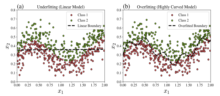
Underfitting occurs when the model is too simple to capture the underlying patterns in the data. In such cases, the model performs poorly on both the training and test datasets. The above Figure(a) illustrates a binary classification model that underfits a complex dataset.

Overfitting occurs when the model is too complex relative to the amount of noise level of the data. In such cases, the model fits the training data very accurately (including its noise) but fails to generalize to unseen data. The above Figure(b) illustrates a binary classification model that overfits a complex dataset.

Both underfitting and overfitting are undesirable in a trained model. The cost function can be used to characterize these behaviors as follows:

1. If both \(\mathcal{C}_{\text{test}}(\boldsymbol{\Theta}^*)\) and \(\mathcal{C}_{\text{train}}(\boldsymbol{\Theta}^*)\) are high, then the model is said to be underfitted.

2. If \(\mathcal{C}_{\text{test}}(\boldsymbol{\Theta}^*)\) is high and \(\mathcal{C}_{\text{train}}(\boldsymbol{\Theta}^*)\) is low, then the model is said to be overfitted.

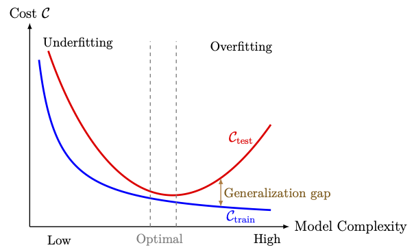Variation of training cost function and test cost function with model complexity, illustrating underfitting, overfitting, and optimal generalization.

Parameter-based Regularization

A neural network with large weights can easily overfit a training dataset. To see this, consider a single neuron with output

\[ y = \mathscr{A}\big(\boldsymbol{w}\cdot \boldsymbol{x} - b\big). \]

If the components of \(\boldsymbol{w}\) are very large, then a small change in \(\boldsymbol{x}\) can lead to a large change in the output \(y\). This makes the neuron very sensitive to the input data. Since the model is trained to represent the training data well, the training error is small. However, small changes in the input (for instance, noisy input) can lead to large deviations in the output, leading to a large testing error. Hence, the model shows poor generalization on unseen data, which corresponds to overfitting.

One way to prevent this is to keep the weights smaller by minimizing (also referred to as penalizing) the norm of the weight vector during training. This can be achieved by minimizing a regularized cost function defined as

\[ \mathcal{C}_{\alpha} (\boldsymbol{\Theta}) = \mathcal{C}(\boldsymbol{\Theta}) + \alpha \Omega(\boldsymbol{\Theta}_{\boldsymbol{w}}), \]

where \(\alpha\ge 0\) is a hyperparameter controlling the strength of penalization, and \(\Omega\) is a regularization function, which is a function of the weights only (denoted by \(\boldsymbol{\Theta}_{\boldsymbol{w}}\)).

Commonly used regularization parameters are the following:

\(\ell^1\)-Regularization: In this case, the regularization function is taken as

\[ \Omega(\boldsymbol{\Theta}_{\boldsymbol{w}}) = \|\boldsymbol{\Theta}_{\boldsymbol{w}}\|_1. \]

\(\ell^2\)-Regularization: In this case, the regularization function is taken as

\[ \Omega(\boldsymbol{\Theta}_{\boldsymbol{w}}) = \frac{1}{2}\|\boldsymbol{\Theta}_{\boldsymbol{w}}\|^2_2. \]

Problem:

Obtain the gradient descent update rule for the regularized cost function with \(\ell^2\)-regularization. Recall that we have derived a similar update rule (with a different loss function) earlier in our course. What was it?

Note:

The \(\ell^2\)-regularization is called Tikhonov regularization or ridge regression. The \(\ell^1\)-regularization is called lasso in statistical learning.

Problem:

Consider the \(\ell^2\)-regularized loss function (used for linear regression)

\[ \mathcal{L}_\alpha(\boldsymbol{w}) = \frac{1}{2}\|\boldsymbol{y} - X\boldsymbol{w}\|_{2}^2 + \frac{\alpha}{2} \| \boldsymbol{w} \|^{2}_{2}, \]

where \(X\) is an \(n\times n\) invertible matrix, and \(\boldsymbol{w},\boldsymbol{y}\in \mathbb{R}^n\). Let \(\boldsymbol{w}^*(\alpha)\) denote the minimizer of the above loss function and let \(c=\|\boldsymbol{w}^*(\alpha)\|^{2}_2\). Then, show that there exists a vector \(\boldsymbol{z}\in \mathbb{R}^n\) such that

\[ c = \sum_{j=1}^n \frac{z_{j}^2}{(\alpha + \lambda_j)^2}, \]

where \(\lambda_j\), \(j=1,2,\ldots, n\), are the eigenvalues of \(X X^\top\).

Remark:

[Constrained Optimization and Geometric Interpretation]

The unconstrained optimization problem with a regularized cost function

\[ \tilde{\boldsymbol{\Theta}} = \text{argmin}_{\boldsymbol{\Theta}}~ \mathcal{C}_{\alpha} (\boldsymbol{\Theta}), \]

for a given \(\alpha>0\), can be equivalently posed as a constrained optimization problem as

\[ \tilde{\boldsymbol{\Theta}} = \left\{\begin{array}{ll} &\displaystyle{\text{argmin}_{\boldsymbol{\Theta}}}~ \mathcal{C}(\boldsymbol{\Theta}),\\ \text{subject to:} & \|\boldsymbol{\Theta}_{\boldsymbol{w}}\|_p \le c, \end{array}\right. \]

for \(p=1,2\), and for some constant \(c\) depending on the regularization parameter \(\alpha\).

Geometric Interpretation:

For the sake of simplicity, let us take \(\boldsymbol{\Theta} = (b,\boldsymbol{w})\) with \(\boldsymbol{w}\in \mathbb{R}^2\), and consider the linear regression model, where the cost function is the MSE function. The regularized minimizer \(\tilde{\boldsymbol{w}}\) corresponds to the point of tangency between the contours (level sets) of the cost surface and the constraint region. The constraint region is a circle (for \(p=2\)) centered at the origin with radius \(c\), as shown in the figure below.

As stated in Problem «Click Here» , for linear regression, in general, we can observe (only numerically) the following dependency between \(\alpha\) and \(c\):

1. as \(\alpha\) increases, \(c\) decreases, and
2. as \(\alpha\) decreases, \(c\) increases.

Hence, choosing a large value of \(\alpha\) makes \(\tilde{\boldsymbol{w}}\) to lie very close to the origin. This leads to a more stable model which is less sensitive to noise but may result in underfitting, with both training and test costs being large. On the other hand, choosing a very small value of \(\alpha\) makes \(\tilde{\boldsymbol{w}}\) to be very close to \(\boldsymbol{w}^*\), often leading to overfitting, where the training error is small but the test error is large, as illustrated in Figure «Click Here» .

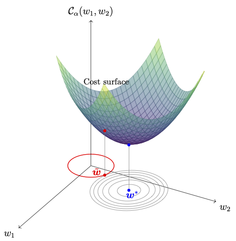Geometric interpretation of \(\ell^2\)-regularized cost function. The 3D surface represents the cost function \(\mathcal{C}_\alpha(\boldsymbol{w})\) as a function of weights \(w_1\) and \(w_2\). The ellipses in the \(w_1\)-\(w_2\) plane show the contour lines of the cost function. The red circle represents the regularization constraint \(\|\boldsymbol{w}\|_2 \leq c\). The unconstrained minimizer \(\boldsymbol{w}^*\) is marked in blue, while the constrained minimizer \(\tilde{\boldsymbol{w}}\) is marked in red, showing the tangency between the constraint and the cost contours.

Process-based Regularization

Process-based regularization techniques work on modifying the training procedure itself to reduce overfitting, rather than directly constraining the model parameters. Some common approaches include early stopping, dropout, data augmentation, and batch normalization. In this subsection, we discuss the early stopping and dropout techniques, and omit the discussion on others.

Early Stopping

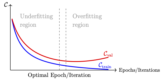
Perhaps, early stopping is the most commonly used regularization technique due to its simplicity and effectiveness. This method monitors the performance of the model on a validation dataset during training and stops the optimization process (in terms of iterations or epoch) when the validation performance ceases to improve.

Recall that the given dataset is divided into three parts, namely, the training dataset, the validation dataset, and the test dataset. The early stopping technique uses the validation dataset to monitor the performance of the model during the training process.

It is generally observed that, as training progresses over iterations or epochs, the training error decreasing monotonically, whereas the validation error shows a different behavior. For the initial iterations (or epochs), the validation error also decreases, but beyond certain point, it starts to increase gradually, producing a U-shape error profile as sketched in the following figure. The early stopping technique makes use of this behavior to decide the stopping criterion for the training process.

An illustrative sketch of the U-shape validation error with the monotonically decreasing training error.

The idea behind the early stopping technique is well understood from the following algorithm:

Algorithm:

[Early Stopping]

Input:

\(\bullet\) Training and validation datasets \(\mathcal{D}_\text{train}\) and \(\mathcal{D}_\text{val}\),

\(\bullet\) Maximum number of epochs/iterations \(K\) (choose this sufficiently large),

\(\bullet\) The number of times the training algorithm has to run before a validation \(n\ll K\),

\(\bullet\) Patience \(p_0\), and

\(\bullet\) Cost/loss function.

Processing:

Assign \(p=0\), and \(\mathcal{C}_{\text{val}}^* = +\infty\) (a sufficiently large number while programming).

Initialize the parameter \(\boldsymbol{\Theta}_0\) (mostly randomly and in some simple cases, take it zero).

Start with \(k=0\) and do the following while \(k\le K\):

Step 1: Train the model by running the epochs/iterations for \(j=1,2,\ldots, n\) using any of the optimization methods that we discussed in the previous section. Assign

\[ k \leftarrow k + n. \]

Let the parameter at the end of this training step be denoted by \(\boldsymbol{\Theta}_k\).

Step 2: Validate \(\boldsymbol{\Theta}_k\) by performing the following steps:

\(~~~~~~\)Step 2A: Perform forward propagation on all the examples of \(\mathcal{D}_\text{val}\),

\(~~~~~~\)Step 2B: Compute \(\mathcal{C}_{\text{val}}\).

\(~~~~~~\)Step 2C: Check the following:

\(~~~~~~~~~~~\) If \(\mathcal{C}_{\text{val}} < \mathcal{C}_{\text{val}}^*\), then assign

\(~~~~~~~~~~~\) \(~~~~\mathcal{C}_{\text{val}}^* = \mathcal{C}_{\text{val}},\)

\(~~~~~~~~~~~\) \(~~~~\tilde{\boldsymbol{\Theta}} = \boldsymbol{\Theta}_k\).

\(~~~~~~~~~~~\) \(~~~~p=0\).

\(~~~~~~~~~~~\) Else

\(~~~~~~~~~~~\) \(~~~~ p \leftarrow p+1.\)

\(~~~~~~~~~~~~~~~\) If \(p \ge p_0\), then stop and go for the output.

\(~~~~~~~~~~~~~~~\) Else, go for the next epoch/iteration.

Output: \(\tilde{\boldsymbol{\Theta}}\).

Note:

1. It is advisable to also tune the learning rate \(\eta\) simultaneously. For instance, when \(p = p_0/2\), the validation performance might improve by reducing the learning rate.

2. The validation frequency \(n\) in the above algorithm is a hyperparameter.

Dropout

As we can see from Figure «Click Here» , increasing the model complexity can lead to overfitting. However, in many practical situations, a high-capacity (more neurons and layers) model is desirable to capture complex patterns in the data. In such cases, dropout serves as an efficient regularization technique to prevent overfitting without substantially reducing model complexity (number of neurons and layers).

Given a neural network, the dropout technique implicitly trains an ensemble of subnetworks where all subnetworks share the same parameter set \(\boldsymbol{\Theta}\).

A subnetwork of a given parent network is obtained by removing a subset of neurons from one or more layers (typically excluding the output layer to preserve valid predictions).

The dropout technique is a training procedure where each iteration of the optimization is performed on a subnetwork which is obtained by dropping out some neurons from said layers (other than the output layer) randomly. The neurons are dropped by multiplying the output of the neurons by a factor \(r\) that takes the value 0 with certain preassigned probability.

First, choose the vector of dropout probabilities \(\boldsymbol{p} = (p^{(0)}, p^{(1)}, \ldots, p^{(L-1)})\), where each \(p^{(l)}\in [0,1)\), for \(l=0,1,2,\ldots, L-1\), is called the dropout probability of the \(l^{\rm th}\) layer.

For each training iteration, a set of mask vectors \(\boldsymbol{r}^{(l)}\), for \(l=0,1,2,\ldots, L-1\), is randomly generated with \(r^{(l)}_i \sim \text{Bernoulli}(1-p^{(l)})\), i.e.,

\[ r^{(l)}_i = \left\{\begin{array}{ll} 0,&\text{with probability}~ p^{l},\\ 1,&\text{with probability}~ 1-p^{l}, \end{array}\right. \quad i=1,2,\dots,n_l. \]

Then, the activation of the \(l^{\rm th}\) layer is redefined as

\[ \tilde{\boldsymbol{a}}^{(l)} = \frac{\boldsymbol{r}^{(l)} \odot \boldsymbol{a}^{(l)}}{1-p^{l}}, \]

where \(\boldsymbol{a}^{(l)}\) is the vector without dropout. Thus, during training, each forward pass effectively uses a different subnetwork, with all subnetworks sharing the same parameter set \(\boldsymbol{\Theta}\).

Note:

It is important to note that dropout procedure is applied only at during training. During testing (inference), the full network is used without dropout, i.e., \(\tilde{\boldsymbol{a}}^{(l)} = \boldsymbol{a}^{(l)}\).

The dropout methodology allows us to implicitly train an ensemble of subnetworks, and it is generally observed to be successful in improving generalization and reducing overfitting without altering the basic architecture of the network.

Problem:

Modify the batch forward propagation Algorithm «Click Here» to incorporate the dropout procedure for a single forward pass.

Generalization

In deep learning, generalization refers to the ability of a model to perform well on an unseen dataset. Recall that before learning a model we consider three datasets, where the training dataset is used to learn the model parameters, the validation dataset is used to tune the hyperparameters during the training process to achieve an optimal trade-off between underfitting and overfitting. Once the model is trained, it is then applied on the test dataset, which is kept unseen during training and is used to evaluate the final performance of the trained model.

Most of the practical situations (if not always), we have

\[ \mathcal{C}_\text{train}(\boldsymbol{\Theta}) \le \mathcal{C}_\text{test}(\boldsymbol{\Theta}). \]

Given the above scenario, if the generalization gap satisfies the inequality

\[ \mathcal{C}_\text{test}(\boldsymbol{\Theta}) - \mathcal{C}_\text{train}(\boldsymbol{\Theta}) < \epsilon, \]

for some pre-assigned number \(\epsilon>0\) and the model achieves a reasonably small training error, then the model is said to generalize well. In this case, the model is expected to perform well on unseen data. This is the desired scenario in deep learning. In this case, we say that the model has learned the underlying patterns in the data rather than memorizing the training examples, which may include noise.

Achieving good generalization depends on appropriately tuning the hyperparameters, such as the complexity of the model (its depth and width), the size and representativeness of the training dataset, and the use of suitable regularization techniques. Although we have good mathematical understanding of the role of these parameters in learning a model, practical success often relies heavily on experience, experimentation, and intuition about their choice. Thus, achieving good generalization is often more of an art than a science. Nevertheless, there are some mathematical principles that can partially guide us towards achieving good generalization. In this section, we discuss one such principle, known as the bias-variance tradeoff.

Bias-Variance Tradeoff

A classical statistical perspective of generalization comes from the bias-variance tradeoff. This perspective is particularly relevant when the cost function is MSE. In this case, the expected cost function can be written as the sum of two opposing terms, namely the bias and the variance.

Assume that \(N\) labeled examples are drawn independently from an unknown joint probability distribution \(p(\boldsymbol{x},\boldsymbol{y})\) to form a training dataset, denoted by \(\mathcal{D}\). In this way, we can have many such training datasets. For each dataset, the learning algorithm produces a predictor (an ANN model in our case), denoted by \(\mathscr{F}_{\mathcal{D}}(\boldsymbol{x})\), which may differ depending on the dataset.

The aim is to design a learning process (by choosing a suitable network with suitably tuned hyperparameters) that can train a predictor capable of generalizing well to unseen test samples \((\boldsymbol{x},\boldsymbol{y})\) drawn from the same distribution.

Clearly, there is a randomness in the way the training datasets are generated. We therefore treat \(\mathcal{D}\) as a random variable representing a training dataset of \(N\) examples. Consequently, the leaned predictor \(\mathscr{F}_{\mathcal{D}}(\boldsymbol{x})\), obtained from a fixed learning algorithm (fixed architecture and a set of hyperparameters), is also a random variable. The generalization performance of these predictors can be assessed by taking an average over a collection of training datasets.

Assume that the true label is generated as

\[ \boldsymbol{y} = \boldsymbol{f}(\boldsymbol{x}) + \boldsymbol{\epsilon}, \]

where \(\boldsymbol{f}\) is the true underlying function to be learnt and \(\boldsymbol{\epsilon}\) is a random noise term with mean \(\mathbb{E}(\boldsymbol{\epsilon}) = \boldsymbol{0}\) and the covariance matrix is denoted by \(\Sigma_\epsilon := \mathrm{Cov}(\boldsymbol{\epsilon})\). This accounts for variability or measurement noise in the data-generating process.

At a given test input \(\boldsymbol{x}\), the expected squared prediction error is given by

\[ \mathbb{E}_{\mathcal{D}, \boldsymbol{y}}\!\left[\|\boldsymbol{y} - \mathscr{F}_{\mathcal{D}}(\boldsymbol{x})\|^2\right] = \mathbb{E}_{\mathcal{D}, \boldsymbol{\epsilon}}\!\left[\|\boldsymbol{f}(\boldsymbol{x}) + \boldsymbol{\epsilon} - \mathscr{F}_{\mathcal{D}}(\boldsymbol{x})\|^2\right], \]

where the expectation is taken jointly over the randomness in both \(\mathcal{D}\) and \(\boldsymbol{y}\), and \(\|\cdot\|\) is the Euclidean norm.

Expanding the square and using \(\mathbb{E}[\boldsymbol{\epsilon}] = \boldsymbol{0}\) and \(\mathbb{E}\!\left[\|\boldsymbol{\epsilon}\|^2\right] = \mathrm{tr}(\Sigma_\epsilon),\) we can derive the decomposition of the total error as

\[ \mathbb{E}_{\mathcal{D}, \boldsymbol{y}}\!\left[\|\boldsymbol{y} - \mathscr{F}_{\mathcal{D}}(\boldsymbol{x})\|^2\right] = \underbrace{\|\mathbb{E}_{\mathcal{D}}[\mathscr{F}_{\mathcal{D}}(\boldsymbol{x})] - \boldsymbol{f}(\boldsymbol{x})\|^2}_{\text{Bias}^2} + \underbrace{\mathbb{E}_{\mathcal{D}}\!\left[\|\mathscr{F}_{\mathcal{D}}(\boldsymbol{x}) - \mathbb{E}_{\mathcal{D}}[\mathscr{F}_{\mathcal{D}}(\boldsymbol{x})]\|^2\right]}_{\text{Variance}} + \underbrace{\mathrm{tr}(\Sigma_\epsilon)}_{\text{Noise}}. \]

Note that the intrinsic uncertainty in the data, represented by \(\mathrm{tr}(\Sigma_\varepsilon)\), is irreducible by any learning algorithm.

Problem:

Give the full derivation of the above expression.

Remark:

[Interpretation]

The left hand side of the above expression is the expected prediction error, which is decomposed into three parts, namely,

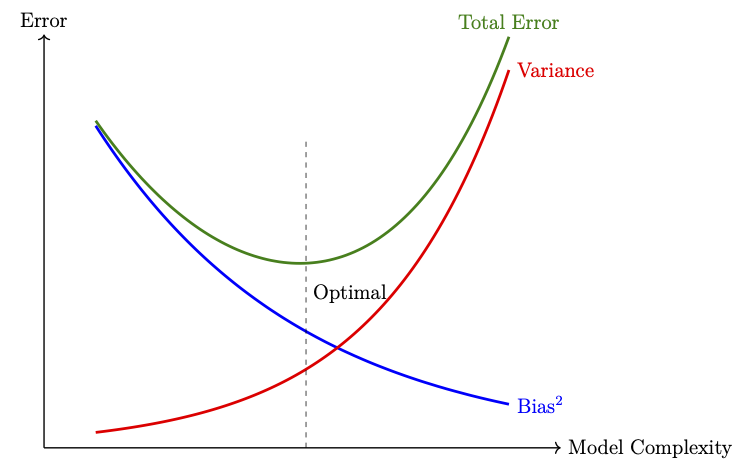
1. Bias\(^2\) measures the squared difference between the average prediction of the model and the true function \(\boldsymbol{f}\). A high bias indicates a systematically wrong model (underfitting).
2. Variance measures how sensitive the model’s prediction is to fluctuations in the training data. High variance corresponds to overfitting.
3. Noise is the irreducible error due to randomness in the data itself. It sets a lower bound on the achievable prediction error.

The above expression explains how prediction error can arise from two opposing sources, namely, high bias, due to an overly simple model that fails to capture data complexity, and high variance, due to a model that is too sensitive to fluctuations of the training dataset.

In practice, increasing model complexity reduces the bias but increases the variance. The optimal generalization performance is achieved at a balance between these two opposing effects, known as the bias-variance tradeoff (see the following figure).

An illustrative sketch of Bias-Variance Tradeoff