Multilayer Perceptrons

So far, we have studied models based on a single neuron. More precisely, from our discussions on perceptrons and their learning algorithms, we see that a single neuron model can learn a linear decision boundary. The same holds for SVMs when we directly apply those models to the dataset in the input space. By defining a suitable feature map to transform the dataset from the input space to a feature space, we can learn datasets that are not linearly separable. However, such feature maps have to be chosen manually (in perceptrons) or through kernel tricks (in SVMs), where the kernel needs to be chosen suitably. Many real-world problems give rise to nonlinearly separable datasets of high dimensions and involve more complex features. In such cases, it is more difficult to specify a feature map manually, and it is desirable to have a model that can learn its own representation directly from the data, which can lead to more accurate classifications.

A multilayer neural network learns complex patterns from a dataset by automatically extracting both the feature representation and the decision boundary. The main idea is to arrange many neurons together to form a layer, with each neuron extracting different features from the input. Further, by stacking multiple layers, the network learns a sequence of nonlinear transformations. For instance, the first layer may capture simple patterns, the next layer may build more complex features from them, further deeper layers may combine these features into highly abstract representations, and finally, the last layer can apply a simple linear classifier to separate the data. In this way, multilayer neural networks overcome the main limitation of single-neuron models and SVMs by learning both the feature representation and the decision boundary simultaneously, and also directly from a dataset.

A multilayer neural network can be viewed as a function that maps an input vector to an output vector. In other words, it implements a mathematical transformation from the input space to the output space. From this perspective, a neural network can be viewed as a universal function approximator, which can approximate an unknown function underlying a given dataset. When the output vector represents real values, the network can be used for regression or function approximation tasks. When the output vector represents class scores or probabilities, the network naturally serves as a classifier.

In this chapter, we introduce fully connected feedforward artificial neural networks (also called the Multilayer Perceptrons (MLPs)) as a natural extension of single-neuron models. In Section «Click Here», we begin with a mathematical definition of MLPs and then discuss the dimensions of weight matrices and bias vectors. We also list some commonly used nonlinear activation functions in Section «Click Here». Using simple illustrations, we demonstrate how activations shape the network’s output and decision boundaries.

Fully Connected Feedforward Networks

An artificial neural network (ANN) is a system consisting of layers of connected neurons that defines a parametric function mapping input vectors to output vectors. The parameters of an ANN are learnt from a dataset through a training process that enables the network to approximate the underlying relationship between the inputs and the outputs.

An ANN is typically organized into three components, namely,

an input layer that receives the input vectors;
a set of hidden layers that perform transformations through affine maps and activation functions; and
an output layer that produces the final prediction or classification.

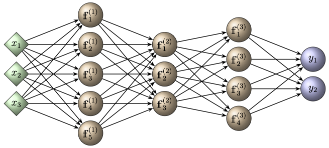
A shallow network refers to a neural network with at most one hidden layer between the input and output. A neural network with two or more hidden layers is considered a deep network.

The multilayered structure of a deep neural network is illustrated in the following figure.

Schematic of an ANN with three hidden (brown) layers. The leftmost (green) layer is the input layer, that receives the input vector, and the rightmost (blue) layer corresponds to the output vector.

Definition and Network Dimensions

Having set the structure of ANNs intuitively, we now turn our attention to give the mathematical definition of a fully connected ANN.

Definition:

[Artificial Neural Network (ANN)]

For a given \(L\in \mathbb{N}\) and a set of network dimensions \(n_0,n_1, n_2, \ldots, n_L\in \mathbb{N}\), a fully connected artificial neural network of depth \(L\) and width \(\hat{n}=\max(n_1, n_2, \ldots, n_{L-1})\), is a parametric function \({\mathscr{F}_{L,\hat{n}}}: \mathbb{R}^{n_0} \rightarrow \mathbb{R}^{n_L}\) defined as

\[ {\mathscr{F}_{L,\hat{n}}}(\boldsymbol{x}; \boldsymbol{\Theta}) =\mathfrak{h}^{(L)} \big( \mathfrak{h}^{(L-1)}\big( \cdots \mathfrak{h}^{(2)} \big(\mathfrak{h}^{(1)} (\boldsymbol{x};\overline{W}^{(1)}); \overline{W}^{(2)} \big)\cdots; \overline{W}^{(L-1)}\big); \overline{W}^{(L)} \big), \]

for all input vectors \(\boldsymbol{x}\in \mathbb{R}^{n_0}\).

Here, for each layer \(l=1,2,\ldots,L\), the layer function \( \mathfrak{h}^{(l)}: \mathbb{R}^{n_{l-1}} \rightarrow \mathbb{R}^{n_{l}}\) is the vector-valued neuron function of the \(l^{\rm th}\) layer

\[ \mathfrak{h}^{(l)} (\boldsymbol{x}^{(l-1)};\overline{W}^{(l)}) = \big( \text{𝕗}_1^{(l)} (\overline{\boldsymbol{x}}^{(l-1)};\overline{\boldsymbol{w}}_1^{(l)}), \ldots, \text{𝕗}_{n_l}^{(l)} (\overline{\boldsymbol{x}}^{(l-1)};\overline{\boldsymbol{w}}_{n_l}^{(l)}) \big)^\top, \]

with each \(\text{𝕗}_{k}^{(l)}: \{-1\}\times \mathbb{R}^{n_{l-1}} \rightarrow \mathbb{R}\) being the neuron function defined in Definition «Click Here», and

\[ \overline{W}^{(l)} = \left[\overline{\boldsymbol{w}}_{1}^{(l)}~ \overline{\boldsymbol{w}}_2^{(l)}~\cdots~\overline{\boldsymbol{w}}_{n_l}^{(l)}\right]^\top, \]

being the \(n_{l} \times (n_{l-1}+1)\) augmented weight matrix, and \(\boldsymbol{\Theta}\) denotes the collection of trainable parameters of the network as

\[ \boldsymbol{\Theta} = \big(\overline{W}^{(1)}, \overline{W}^{(2)}, \ldots, \overline{W}^{(L)}\big). \]

The layer corresponding to \(l=0\) is the input layer, and the layer with \(l=L\) is the output layer, whereas the layers for \(l=1,2,\ldots, L-1\) are the hidden layers with layer width \(n_l\).

Note:

Neurons in the hidden and output layers are often referred to as units or nodes.

The input vectors are augmented only at the neuron level while computing the neuron functions. Whereas, the layer functions take the raw input vectors as arguments and produce outputs without bias augmentation.

The width of the \(l^{\rm th}\) hidden layer is \(n_l\).

Remark:

In a simple notation, we may write

\begin{eqnarray} {\mathscr{F}_{L,\hat{n}}} = \mathfrak{h}^{(L)} \circ \mathfrak{h}^{(L-1)} \circ \ldots \circ \mathfrak{h}^{(2)} \circ \mathfrak{h}^{(1)}, \end{eqnarray}

(4.1)

which is a mapping \(\mathbb{R}^{n_0} \ni \boldsymbol{x} \mapsto \boldsymbol{y}\in \mathbb{R}^{n_L}\) obtained by passing the input vector \(\boldsymbol{x}\) successively through the hidden layers, starting from layer \(l=1\) up to layer \(l=L-1\), and finally through the output layer \(l=L\) to obtain the output vector \(\boldsymbol{y}\). Such a network is also called a feedforward neural network. A fully connected (or densely connected) feedforward neural network defined above is often referred to as a multilayer perceptron (MLP).

Note:

In the Chapter «Click Here» on Perceptron, we defined a perceptron as a single neuron with the Heaviside (or bipolar) activation function. In contrast, in the context of neural networks, a multilayer perceptron may involve any of the commonly used activation functions in its neuron functions, and is not restricted to the Heaviside (or bipolar) choice.

Problem:

Find the network dimensions, width, and depth of the MLP shown in the above Figure «Click Here» . Also, find the total number of parameters (weights and bias) involved in the network.

Training or learning an artificial neural network means obtaining a collection of trainable parameters \(\boldsymbol{\Theta}\) by optimizing a suitable cost function over the given training dataset. Recall the learning process as briefed in Subsection «Click Here» (in the context of supervised learning).

Shallow Networks

From Definition «Click Here» , we see that an ANN is defined as a composition of layers, where each layer applies an affine transformation followed by a nonlinear activation function. In this subsection, we construct an explicit form of a shallow network with one hidden layer, that is, \(L=2\).

Let the network dimensions be \(n_0, n_1, n_2\in \mathbb{N}\). From Definition «Click Here» , a shallow network with width \(\hat{n}=n_1\) is a function \({\mathscr{F}_{2,\hat{n}}}:\mathbb{R}^{n_0}\rightarrow \mathbb{R}^{n_2}\) given by

\begin{eqnarray} {\mathscr{F}_{2,\hat{n}}} (\boldsymbol{x};\boldsymbol{\Theta}) = \mathfrak{h}^{(2)}\big(\mathfrak{h}^{(1)} (\boldsymbol{x};\overline{W}^{(1)});\overline{W}^{(2)}\big),~\boldsymbol{x}\in \mathbb{R}^{n_0}. \end{eqnarray}

(4.2)

The augmented weight matrices are given by

\begin{eqnarray} \overline{W}^{(l)} = \left(\begin{array}{llllcl} b^{(l)}_1&w^{(l)}_{11}&w^{(l)}_{12}&\cdots&w^{(l)}_{1n_{l-1}}\\ b^{(l)}_2&w^{(l)}_{21}&w^{(l)}_{22}&\cdots&w^{(l)}_{2n_{l-1}}\\ \ldots & & \cdots &\cdots&\cdots\\ \ldots & & \cdots &\cdots&\cdots\\ \ldots & & \cdots &\cdots&\cdots\\ b^{(l)}_{n_{l}}&w^{(l)}_{n_{l}1}&w^{(l)}_{n_{l}2}&\cdots&w^{(l)}_{n_{l}n_{l-1}}\\ \end{array}\right), \end{eqnarray}

(4.3)

for \(l=1,2\). We also write

\begin{eqnarray} \overline{W}^{(l)} = [\boldsymbol{b}^{(l)}~W^{(l)}], ~ \text{where}~ \boldsymbol{b}^{(l)}= \left(\begin{array}{l} b^{(l)}_1\\b^{(l)}_2\\ \cdot\\ \cdot \\ \cdot \\ b^{(l)}_{n_1} \end{array}\right), ~ {W}^{(l)} = \left(\begin{array}{lllcl} w^{(l)}_{11}&w^{(l)}_{12}&\cdots&w^{(l)}_{1n_{l-1}}\\ w^{(l)}_{21}&w^{(l)}_{22}&\cdots&w^{(l)}_{2n_{l-1}}\\ \ldots & \cdots &\cdots&\cdots\\ \ldots & \cdots &\cdots&\cdots\\ \ldots & \cdots &\cdots&\cdots\\ w^{(l)}_{n_{l}1}&w^{(l)}_{n_{l}2}&\cdots&w^{(l)}_{n_{l}n_{l-1}}\\ \end{array}\right). \end{eqnarray}

(4.4)

From Definition «Click Here», the \(k^{\rm th}\) neuron of the \(l^{\rm th}\) layer is given by

\[ \text{𝕗}^{(l)}_k (\overline{\boldsymbol{x}}^{(l-1)};\overline{\boldsymbol{w}}^{(l)}_k) = \mathscr{A}^{(l)}\big(\text{𝕒}(\overline{\boldsymbol{x}}^{(l-1)};\overline{\boldsymbol{w}}^{(l)}_k) \big), ~l=1,2,~k=1,2,\ldots, n_{l}, \]

where \(\overline{\boldsymbol{w}}^{(l)}_k = (b^{(l)}_k, w^{(l)}_{k1}, w^{(l)}_{k2}, \ldots, w^{(l)}_{kn_{l-1}})^\top\) and \(\overline{\boldsymbol{x}}^{(l-1)} = (-1, \boldsymbol{x}^{(l-1)})^\top\) are the augmented weight and input (column) vectors, respectively, \(\text{𝕒}:\{-1\}\times \mathbb{R}^{n_{l-1}}\rightarrow \mathbb{R}\) is the affine function given by

\[ \text{𝕒}(\overline{\boldsymbol{x}}^{(l-1)};\overline{\boldsymbol{w}}^{(l)}_k) = \big\langle \overline{\boldsymbol{w}}^{(l)}_k, \overline{\boldsymbol{x}}^{(l-1)} \big\rangle, \]

and \(\mathscr{A}^{(l)}: \mathbb{R} \rightarrow \mathbb{R}\) is the nonlinear activation function used in the \(l^{\rm th}\) layer.

For \(l=1\), \(\boldsymbol{x}^{(0)} = \boldsymbol{x}\in \mathbb{R}^{n_0}\) is the input vector, and for \(l=2\), \(\boldsymbol{x}^{(1)}\in \mathbb{R}^{n_1}\) is the output of the first layer given by

\[ \boldsymbol{x}^{(1)} = \mathfrak{h}^{(1)} (\boldsymbol{x}^{(0)};\overline{W}^{(1)}), \]

which is often referred to as the activation of that layer. Finally, at the output, we have

\[ \boldsymbol{y} = \mathfrak{h}^{(2)} (\boldsymbol{x}^{(1)};\overline{W}^{(2)}). \]

Note:

It is important to note that at each layer, the input is taken without augmentation. Whereas, the augmentation is done only within the affine function, where we take the inner product (which is just a dot product in a finite-dimensional vector space) of the augmented input and weight vectors.

Remark:

Although it is mathematically possible to assign different activation functions to different neurons within the same layer, such a network complicates both the learning process and the mathematical analysis. A common practice is to use the same activation function for all neurons in a hidden layer, and a different one for the output layer, if required. This distinction is often essential, as different tasks need different forms of the output. For instance, function approximation (regression) often uses a linear activation, binary classification may use thresholding functions like Heaviside or bipolar (historically), or their smoother versions like sigmoid or tanh (to be introduced in the next subsection), and multi-class classification requires the softmax activation.

For notational convenience, we introduce the vector notation for the affine transformation and the activation function.

Remark:

[Vector form of an activation]

We define the affine function of the \(l^{\rm th}\) layer as the vector-valued function \(\underline{𝕒}:\{-1\}\times \mathbb{R}^{n_{l-1}} \rightarrow \mathbb{R}^{n_l}\) given by

\begin{eqnarray} \underline{𝕒}(\overline{\boldsymbol{x}}^{(l-1)};\overline{W}^{(l)}) &=& \overline{W}^{(l)}\overline{\boldsymbol{x}}^{(l-1)}\\ &=& W^{(l)}\boldsymbol{x}^{(l-1)} - \boldsymbol{b}^{(l)}, \end{eqnarray}

(4.5)

where \(\boldsymbol{x}^{(l-1)}\in \mathbb{R}^{n_{l-1}}\) is the activation of the \((l-1)^{\rm st}\) layer, \(\boldsymbol{b}^{(l)}\in \mathbb{R}^{n_l}\) is the bias vector, and \(W^{(l)}\) is the \(n_l\times n_{l-1}\) weight matrix of the \(l^{\rm th}\) layer.

For a given activation function \(\mathscr{A}^{(l)}: \mathbb{R}\rightarrow \mathbb{R}\), we define the coordinatewise activation \(\underset{\overline{~~~~}}{\mathscr{A}}^{(l)}:\mathbb{R}^{n_l}\rightarrow \mathbb{R}^{n_l}\) as

\[ \underset{\overline{~~~~}}{\mathscr{A}}^{(l)}(\boldsymbol{x}) = \big(\mathscr{A}^{(l)}(x_1), \mathscr{A}^{(l)}(x_2), \ldots, \mathscr{A}^{(l)}(x_{n_l})\big)^\top, ~\boldsymbol{x}\in \mathbb{R}^{n_l}, \]

where \(\boldsymbol{x}=(x_1,x_2,\ldots, x_{n_l})^\top.\)

Thus, the activation of the \(l^{\rm th}\) layer is the vector \(\boldsymbol{x}^{(l)}\in \mathbb{R}^{n_l}\) given by

\begin{eqnarray} \boldsymbol{x}^{(l)} &=& \mathfrak{h}^{(l)} (\boldsymbol{x}^{(l-1)};\overline{W}^{(l)})\\ &=& \underset{\overline{~~~~}}{\mathscr{A}}^{(l)}\big( \underline{𝕒}(\overline{\boldsymbol{x}}^{(l-1)};\overline{W}^{(l)})\big). \end{eqnarray}

(4.6)

Schematic of single layer neural networks. (a) A real-valued neural network; (b) A vector-valued network.

Example:

Illustrations of single-layer neural networks, with scalar-valued and vector-valued outputs, are depicted in Figure «Click Here» (a) and Figure «Click Here» (b), respectively.

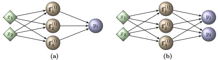
Let us write the explicit form of the ANN shown in Figure «Click Here» (a). The input layer has two features, i.e., \(n_0=2\). There are two layers with the hidden layer having \(n_1=3\) neurons. Thus, the depth of the network is 2 and the width is 3. Therefore, the ANN is the function \({\mathscr{F}_{2,3}}:\mathbb{R}^2\rightarrow \mathbb{R}\) with the trainable parameter

\[ \boldsymbol{\Theta} = \big( \overline{W}^{(1)}, \overline{W}^{(2)} \big), \]

where

\[ \overline{W}^{(1)} = \left(\begin{array}{lll} b^{(1)}_1 & w^{(1)}_{11}& w^{(1)}_{12}\\ b^{(1)}_2 & w^{(1)}_{21}& w^{(1)}_{22}\\ b^{(1)}_3 & w^{(1)}_{31}& w^{(1)}_{32} \end{array}\right),~~ \overline{W}^{(2)} = \left(\begin{array}{llll} b^{(2)}_1 & w^{(2)}_{11}& w^{(2)}_{12}& w^{(2)}_{13} \end{array}\right). \]

The affine function of the first layer is

\[ \underline{𝕒}(\overline{\boldsymbol{x}}^{(0)};\overline{W}^{(1)}) = W^{(1)}\boldsymbol{x}^{(0)} - \boldsymbol{b}^{(1)}, \]

Using the notations in (4.4), we obtain

\begin{eqnarray} \underline{𝕒}(\overline{\boldsymbol{x}}^{(0)};\overline{W}^{(1)}) &=& \left(\begin{array}{ll} w^{(1)}_{11}& w^{(1)}_{12}\\ w^{(1)}_{21}& w^{(1)}_{22}\\ w^{(1)}_{31}& w^{(1)}_{32} \end{array}\right) \left(\begin{array}{l} x^{(0)}_1 \\ x^{(0)}_2 \end{array}\right) - \left(\begin{array}{l} b^{(1)}_1 \\ b^{(1)}_2 \\ b^{(1)}_3 \end{array}\right)\\ &=& \left(\begin{array}{l} w^{(1)}_{11}x^{(0)}_1 + w^{(1)}_{12}x^{(0)}_2- b^{(1)}_1 \\ w^{(1)}_{21}x^{(0)}_1 + w^{(1)}_{22}x^{(0)}_2- b^{(1)}_2 \\ w^{(1)}_{31}x^{(0)}_1 + w^{(1)}_{32}x^{(0)}_2- b^{(1)}_3 \end{array}\right). \end{eqnarray}

(4.7)

The activation \(\boldsymbol{x}^{(1)}\) of the hidden layer is now obtained by applying the activation function \(\mathscr{A}^{(1)}\) of the first hidden layer on the above vector coordinatewise to get

\begin{eqnarray} \boldsymbol{x}^{(1)} &=& \underset{\overline{~~~~}}{\mathscr{A}}^{(1)}\left(W^{(1)}\boldsymbol{x}^{(0)} - \boldsymbol{b}^{(1)}\right)\\ &=&\left(\begin{array}{c} \mathscr{A}^{(1)}\big( w^{(1)}_{11}x^{(0)}_1 + w^{(1)}_{12}x^{(0)}_2- b^{(1)}_1 \big)\\ \mathscr{A}^{(1)}\big( w^{(1)}_{21}x^{(0)}_1 + w^{(1)}_{22}x^{(0)}_2- b^{(1)}_2 \big)\\ \mathscr{A}^{(1)}\big( w^{(1)}_{31}x^{(0)}_1 + w^{(1)}_{32}x^{(0)}_2- b^{(1)}_3 \big) \end{array}\right). \end{eqnarray}

(4.8)

Taking \(\boldsymbol{x}^{(1)}\) as the input, the output is then computed at the output layer as

\[ y = \mathscr{A}^{(2)} \big( w^{(2)}_{11} x^{(1)}_{1} + w^{(2)}_{12} x^{(1)}_{2} + w^{(2)}_{13} x^{(1)}_{3} - b^{(2)}_1 \big). \]

Observe that the right hand side of the above expression is the ANN \({\mathscr{F}_{2,3}}(\cdot\,;\boldsymbol{\Theta})\) of the network depicted in Figure «Click Here» (a) given by (4.2), and its explicit expression is given by \begin{multline*} {\mathscr{F}_{2,3}}(\boldsymbol{x}^{(0)};\boldsymbol{\Theta}) = \mathscr{A}^{(2)}\Big( w^{(2)}_{11}\mathscr{A}^{(1)}\big( w^{(1)}_{11}x^{(0)}_1 + w^{(1)}_{12}x^{(0)}_2- b^{(1)}_1 \big)\\ + w^{(2)}_{12}\mathscr{A}^{(1)}\big( w^{(1)}_{21}x^{(0)}_1 + w^{(1)}_{22}x^{(0)}_2- b^{(1)}_2 \big)\\ + w^{(2)}_{13} \mathscr{A}^{(1)}\big( w^{(1)}_{31}x^{(0)}_1 + w^{(1)}_{32}x^{(0)}_2- b^{(1)}_3 \big) - b^{(2)}_1 \Big), \end{multline*} for every input vector \( \boldsymbol{x}^{(0)}\in \mathbb{R}^{2}\). The network has 13 trainable parameters given by

\[ \boldsymbol{\Theta} = \left( \left(\begin{array}{lll} b^{(1)}_1& w^{(1)}_{11}& w^{(1)}_{12}\\ b^{(1)}_2& w^{(1)}_{21}& w^{(1)}_{22}\\ b^{(1)}_3& w^{(1)}_{31}& w^{(1)}_{32} \end{array}\right) , ~~ \left(\begin{array}{llll} b^{(2)}_1& w^{(2)}_{11}& w^{(2)}_{12}& w^{(2)}_{13} \end{array}\right)\right). \]

Problem:

Derive the explicit expression for the ANN \({\mathscr{F}_{2,3}}(\overline{\boldsymbol{x}}^{(0)};\boldsymbol{\Theta})\) of the network depicted in Figure «Click Here» (b) and give all the trainable parameters of this network.

Batch Forward Propagation

The shallow network computations described in the previous subsection can be generalized to neural networks of arbitrary depth.

For fixed parameters \(\boldsymbol{\Theta}\), the network function \({\mathscr{F}_{L,\hat{n}}}:\mathbb{R}^{n_0}\rightarrow \mathbb{R}^{n_L}\) is well-defined. For every input vector \(\boldsymbol{x}\in\mathbb{R}^{n_0}\), the final output \(\boldsymbol{y}={\mathscr{F}_{L,\hat{n}}}(\boldsymbol{x}; \boldsymbol{\Theta})\) is evaluated recursively by taking the output of the \((l-1)^{\rm st}\) layer as the input to the \(l^{\rm th}\) layer, and computing

\[ \boldsymbol{x}^{(l)} = \mathfrak{h}^{(l)} \big( \boldsymbol{x}^{(l-1)};\overline{W}^{(l)} \big),~l = 1,2,\ldots, L, \]

where \(\boldsymbol{x}^{(l)}\) is called the activation of the \(l^{\rm th}\) layer. This recursive evaluation procedure is referred to as the forward propagation of the activations.

Batch Propagation

Given a dataset

\[ \mathcal{D} = \big\{(\boldsymbol{x}_k, \boldsymbol{y_k}) \mid k=1,2,\ldots, N\big\}\subset \mathbb{R}^{n_0}\times \mathbb{R}^{n_L}, \]

arrange the input vectors in the \(n_0\times N\) matrix form as

\[ {A}^{(0)}:= [ \boldsymbol{x}_1~\boldsymbol{x}_2~\cdots~\boldsymbol{x}_N] = \left(\begin{array}{lllcl} x^{(0)}_{11}&x^{(0)}_{12}&\cdots&x^{(0)}_{1N}\\ x^{(0)}_{21}&x^{(0)}_{22}&\cdots&x^{(0)}_{2N}\\ \ldots &\cdots &\cdots & \cdots \\ \ldots &\cdots &\cdots & \cdots \\ x^{(0)}_{n_01}&x^{(0)}_{n_02}&\cdots&x^{(0)}_{n_0N}\\ \end{array}\right), \]

where each column corresponds to one sample.

To gain computational efficiency, it is preferable to perform forward propagation on the entire dataset in matrix form, rather than evaluating the ANN separately for each input vector.

Then the affine function takes the form

\[ \underline{𝕒}(\overline{A}^{(0)}; \overline{W}^{(1)}) = \overline{W}^{(1)}\overline{A}^{(0)}, \]

where \(\overline{A}^{(0)}\) is the augmented input matrix and the right hand side is a \(n_1\times N\) matrix.

Apply the activation function \(\underset{\overline{~~~~}}{\mathscr{A}}^{(1)}\) to get the activation matrix of the first layer as

\[ A^{(1)} =\underset{\overline{~~~~}}{\mathscr{A}}^{(1)}\big(\overline{W}^{(1)}\overline{A}^{(0)}\big). \]

Taking the activation \(A^{(1)}\) of the first layer as the input to the second layer, the activation of the second layer is computed using the formula

\[ A^{(2)} =\underset{\overline{~~~~}}{\mathscr{A}}^{(2)}\big(\overline{W}^{(2)}\overline{A}^{(1)}\big). \]

Proceed recursively as

\[ A^{(l)} = \underset{\overline{~~~~}}{\mathscr{A}}^{(l)}\big(\overline{W}^{(l)}\overline{A}^{(l-1)}\big), \quad l=1,2,\ldots,L. \]

In general, we have the following algorithm:

Algorithm:

[Batch Forward Propagation]

Input:

Given the trained parameters

\[ \boldsymbol{\Theta} = \big( \overline{W}^{(1)}, \overline{W}^{(2)}, \cdots, \overline{W}^{(L)} \big) \]

Given the dataset in the form of a \(n_0\times N\) matrix \( A^{(0)}. \)

Processing:

For each layer \(l=1,2,\ldots, L\), perform the following computation:

Augment the activation \(A^{(l-1)}\) matrix to obtain \(\overline{A}^{(l-1)}\).

Perform the matrix multiplication

\[ Z^{(l)} = \overline{W}^{(l)}\,\overline{A}^{(l-1)} \]

Apply the activation function to each element of the matrix \(Z^{(l)}\) as follows:

For \(i=1,2,\ldots, n_l\)

For \(j=1, 2, \ldots, N\)

\(A^{(l)}_{ij} = \mathscr{A}^{(l)}(Z^{(l)}_{ij}).\)

Output: \(Y = A^{(L)},\) which is a \(n_L\times N\) matrix

A visualization of the above algorithm is shown in Figure «Click Here»

Visualization of batch forward propagation in a feedforward neural network, showing how the input passes through hidden layers to generate the final output.

Remark:

An artificial neural network can also be uniquely identified by the tuple

\[ \big( \boldsymbol{\Theta}, \underset{\overline{~~~~}}{\mathscr{A}} \big) := \Big((\overline{W}^{(1)}, \underset{\overline{~~~~}}{\mathscr{A}}^{(1)}_{n_1}), (\overline{W}^{(2)}, \underset{\overline{~~~~}}{\mathscr{A}}^{(2)}_{n_2}),\ldots, (\overline{W}^{(L)}, \underset{\overline{~~~~}}{\mathscr{A}}^{(L)}_{n_L})\Big), \]

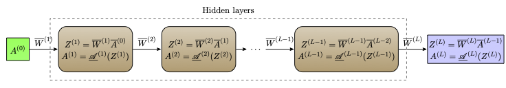
where \(\underset{\overline{~~~~}}{\mathscr{A}}^{(l)}_{n_l}\) denotes the activation function of the \(l^{\rm th}\) layer with the indication of the width of the layer as the suffix.

Code:

\(~\)

Understand the following python code implementing the above forward propagation algorithm:
BatchForwardPropagationDirectImplementation
Understand the following python code that implements forward propagation using TensorFlow-Keras:
BatchForwardPropagationTensorFlow-Keras
In the TensorFlow-Keras implementation of a feedforward neural network, the weights, biases, and batch input \(A^{(0)}\) are handled differently rather than the augmented matrix formats we used in the theoretical formulation.
1. Describe how Keras stores the weight matrices and bias vectors for each layer, and compare this with the augmented weight matrix format \(W^{(l)}\) we used in theory.
2. Explain the difference between the batch input format of \(A^{(0)}\) in Keras (i.e., NumPy/TensorFlow arrays) and the format we used in the theoretical framework (column-wise arrangement of samples) as well as in the first code above.
Understand the following python code that implements forward propagation using PyTorch
BatchForwardPropagationPyTorch
Explain the weight matrix and biases formats of PyTorch and do a similar comparison between PyTorch format and our theoretical formulation as asked in Question 3 above.

Activation Functions

The learning efficiency and the model performance of an ANN depend crucially on the choice of an activation function. In this subsection, we introduce a few commonly used activation functions. For clarity of exposition, we illustrate them using single neurons and shallow networks.

Step Functions

Let us start our discussion with a class of activation functions that we are already familiar from our discussions in the previous chapters.

Heaviside function

Unit step function of the Heaviside function is called the threshold activation function, given by

\begin{eqnarray} \mathscr{H}(x) = \left\{\begin{array}{lc} 0,&\text{if}~x<0\\ 1,&\text{if}~x\ge 0 \end{array}\right. \end{eqnarray}

(4.9)

In terms of distributional derivatives, the derivative of the Heaviside function is given by \(\mathscr{H}'(x) = \delta(x)\), where \(\delta\) denotes the Dirac's measure.

Bipolar Function

The bipolar function is called the bipolar activation function and is given by

\begin{eqnarray} \mathscr{B}(x) = \left\{\begin{array}{rc} -1,&\text{if}~x<0\\ 1,&\text{if}~x\ge 0 \end{array}\right. \end{eqnarray}

(4.10)

It is easy to see that \(\mathscr{B}(x) = 2\mathscr{H}(x) - 1\). Therefore, the distributional derivative of \(\mathscr{B}\) is given by \(\mathscr{B}'(x) = 2\delta(x)\).

The threshold and bipolar activation functions are used at the output layer of problems involving binary classification, which we studied in the context of perceptrons in the Chapter «Click Here».

Sigmoid Functions: Logistic Regression

A sigmoid function is a continuously differentiable function \(\mathscr{S}:\mathbb{R} \rightarrow (0,1)\), such that \(\mathscr{S}'>0\) (strictly increasing) and \(\mathscr{S}(s)\rightarrow 0\) as \(s\rightarrow -\infty\) and \(\mathscr{S}(s)\rightarrow 1\) as \(s\rightarrow +\infty\).

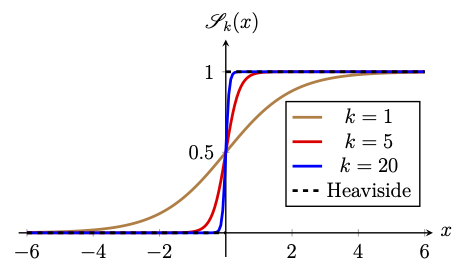
A commonly used sigmoid function is the logistic function with parameter \(k>0\) and is defined as

\begin{eqnarray} \mathscr{S}_k(s) = \frac{1}{1+e^{-ks}}, ~ s\in \mathbb{R}. \end{eqnarray}

(4.11)

The graphs of the sigmoid function for various values of \(k\) are depicted in the following figure. From the figure, we observe that \(\mathscr{S}_k\rightarrow \mathscr{H}\) pointwise as \(k\rightarrow \infty\) on \(\mathbb{R}\backslash \{0\}\).

Graphs of the logistic sigmoid function for various values of \(k\), illustrating convergence to the Heaviside step function as \(k \to \infty\).

Since we use gradient-based optimization methods (such as gradient descent method) for learning a neural network, smooth activation functions like the logistic function are preferred over the Heaviside function, which is non-differentiable and constant almost everywhere. Moreover, the logistic function maps \(x \mapsto y \in (0,1)\) and hence its output can be interpreted as a probability. This makes it particularly useful in probabilistic models such as logistic regression.

Example:

[Logistic Regression]

Consider a dataset

\[ \mathcal{D} = \big(\mathcal{C}^-\times \{0\}\big) \cup \big(\mathcal{C}^+\times \{1\}\big). \]

If \(\mathcal{D}\) is linearly separable, then a perceptron can learn a separating hyperplane with weight \(\boldsymbol{w}\) and bias \(b\), and classify inputs by the rule

\[ \hat{y} = \begin{cases} 1, & \langle \boldsymbol{w}, \boldsymbol{x}\rangle - b > 0, \\ 0, & \text{otherwise}. \end{cases} \]

This is a hard classification rule that outputs only \(0\) or \(1\).

Instead of making a hard decision, we may ask the following question:

What is the probability that an input \(\boldsymbol{x}\) belongs to \(\mathcal{C}^+\)?

Using Bayes’ theorem, the posterior probability for the class \(\mathcal{C}^+\) can be written as

\[ \mathbb{P}(\mathcal{C}^+ \mid \boldsymbol{x}) = \frac{p(\boldsymbol{x} \mid \mathcal{C}^+) \mathbb{P}(\mathcal{C}^+)} {p(\boldsymbol{x} \mid \mathcal{C}^+) \mathbb{P}(\mathcal{C}^+) + p(\boldsymbol{x} \mid \mathcal{C}^-) \mathbb{P}(\mathcal{C}^-)}, \]

where \(\mathbb{P}\) denotes a probability measure, and \(p\) is the probability mass (or density) function associated with \(\mathbb{P}\).

Taking the ratio of posteriors, we get

\[ \frac{\mathbb{P}(\mathcal{C}^+ \mid \boldsymbol{x})}{\mathbb{P}(\mathcal{C}^- \mid \boldsymbol{x})} = \frac{p(\boldsymbol{x} \mid \mathcal{C}^+) \mathbb{P}(\mathcal{C}^+)}{p(\boldsymbol{x} \mid \mathcal{C}^-) \mathbb{P}(\mathcal{C}^-)}, \]

which is referred to as the odds. The logarithm of the odds is called the logit or log-odds, and from the above expression, we see that the log-odds can be written as

\[ \log \frac{\mathbb{P}(\mathcal{C}^+ \mid \boldsymbol{x})}{\mathbb{P}(\mathcal{C}^- \mid \boldsymbol{x})} = \log \Lambda(\boldsymbol{x}) + \log\left( \frac{\mathbb{P}(\mathcal{C}^+)}{\mathbb{P}(\mathcal{C}^-)}\right), \]

where

\[ \Lambda(\boldsymbol{x}) = \frac{p(\boldsymbol{x} \mid \mathcal{C}^+)}{p(\boldsymbol{x} \mid \mathcal{C}^-)} \]

is the likelihood ratio.

Assume that the log-likelihood ratio is linear in \(\boldsymbol{x}\), that is, there is a weight vector \(\boldsymbol{w}\) such that

\[ \log \Lambda(\boldsymbol{x}) = \langle \boldsymbol{w}, \boldsymbol{x} \rangle, \]

for all input vectors \(\boldsymbol{x}\). Then the log-odds can be written as

\[ \log \frac{\mathbb{P}(\mathcal{C}^+ \mid \boldsymbol{x})}{\mathbb{P}(\mathcal{C}^- \mid \boldsymbol{x})} = \langle \boldsymbol{w}, \boldsymbol{x} \rangle - b, \]

where \(b = - \log\left( \tfrac{\mathbb{P}(\mathcal{C}^+)}{\mathbb{P}(\mathcal{C}^-)}\right)\) is treated as the bias.

Noting that \(\mathbb{P}(\mathcal{C}^- \mid \boldsymbol{x}) = 1 - \mathbb{P}(\mathcal{C}^+ \mid \boldsymbol{x})\) and solving the above equation for \(\mathbb{P}(\mathcal{C}^+ \mid \boldsymbol{x})\), we obtain

\[ \mathbb{P}(\mathcal{C}^+ \mid \boldsymbol{x}) = \mathscr{S}_1\big(\langle \boldsymbol{w}, \boldsymbol{x} \rangle - b\big). \]

The interpretation of the above expression is as follows:

Given an input vector \(\boldsymbol{x}\), the probability that it belongs to the class \(\mathcal{C}^+\) is equal to the value of the logistic function \(\mathscr{S}_1\) at the point \(s = \langle \boldsymbol{w}, \boldsymbol{x} \rangle - b\).

Thus, estimating a weight vector \(\boldsymbol{w}\) and a bias \(b\) allows us to assign probabilities for each of the two classes \(\mathcal{C}^+\) and \(\mathcal{C}^-\). At the inference stage, by applying a suitable decision rule (for instance, thresholding at \(0.5\)), we obtain a binary (hard) classification. In the context of statistical learning, such a probabilistic classification model is called logistic regression.

Problem:

Show that \(\mathscr{S}_1^{-1}\) is the logit or log-odd function.

Remark:

[Neuron Viewpoint of Logistic Regression]

Logistic regression can be viewed as a single artificial neuron with the neuron function as

\[ \text{𝕗}^{(1)}(\overline{\boldsymbol{x}}^{(0)};\overline{\boldsymbol{w}}^{(1)}) = \mathscr{S}_1 \big( \text{𝕒}(\overline{\boldsymbol{x}}^{(0)};\overline{\boldsymbol{w}}^{(1)}) \big), \]

for any given input vector \(\overline{\boldsymbol{x}}^{(0)}\in \mathbb{R}^{n_0}\). Thus, logistic regression can be trained as an artificial neuron to approximate the posterior probability of the positive class of a given dataset, so that the output is

\[ \hat{p} = \mathbb{P}(\mathcal{C}^+ \mid \boldsymbol{x}). \]

Hard classification is then obtained during inference by applying a decision rule

\[ \hat{y} = \begin{cases} 1, & \text{if} ~ \hat{p} \ge \hat{p}^*, \\ 0, & \text{otherwise}, \end{cases} \]

where \(\hat{p}^*\in (0,1)\) is chosen based on applications. For instance, \(\hat{p}^*=0.5\) is a default choice.

Note:

Logistic regression finds the best linear boundary in a probabilistic sense that provides a measure of confidence. Hard classification is obtained only at the inference stage by applying a decision rule (e.g., thresholding). Because of this probabilistic formulation, logistic regression can also be applied to datasets that are not linearly separable.

Recall from the Subsection «Click Here» on Supervised Learning that to learn parameters \((b, \boldsymbol{w})\) of a model, we have to choose a suitable cost function. There is a natural choice of the cost function to train logistic regression, which we discuss in the following remark.

Remark:

[Cross-entropy Cost Function]

A natural training principle for logistic regression is to maximize the likelihood that the model assigns to the observed labels, given the predicted probabilities. Let us make this idea more precise:

For a single training example \((\boldsymbol{x}_i,y_i)\), the model predicts a probability \(\hat{p}_i = P(\mathcal{C}^+ \mid \boldsymbol{x}_i)\). The likelihood of observing the true label \(y_i \in \{0,1\}\) under this prediction is

\[ L_i = \hat{p}_i^{\,y_i}\,(1-\hat{p}_i)^{\,1-y_i}. \]

For an entire training dataset \(\mathcal{D}_\text{train} = \big\{(\boldsymbol{x}_i,y_i) \mid i=1,2,\ldots, N_\text{train}\big\}\) having independent samples (examples) from the underlying joint distribution, the joint likelihood is the product

\[ L(b, \boldsymbol{w}) = \prod_{i=1}^{N_\text{train}} \hat{p}_i^{y_i} (1 - \hat{p}_i)^{1-y_i}. \]

Rather than maximizing this product directly, it is more convenient to work with the log-likelihood

\[ \log L(b, \boldsymbol{w}) = \sum_{i=1}^{N_\text{train}} \Big[ y_i \log \hat{p}_i + (1-y_i)\log(1-\hat{p}_i) \Big]. \]

Thus, the training objective for logistic regression is to maximize the log-likelihood. Equivalently, minimizing the negative log-likelihood yields the cross-entropy cost function, given by

\begin{eqnarray} \mathcal{L}(b, \boldsymbol{w}) = - \frac{1}{N_\text{train}}\sum_{i=1}^{N_\text{train}} \Big[ y_i \log \hat{p}_i + (1-y_i)\log(1-\hat{p}_i) \Big]. \end{eqnarray}

(4.12)

The cost function \(\mathcal{L}(\boldsymbol{w}, b)\) is smooth and convex, but it has no closed-form solution. The most suitable optimization algorithm is gradient descent (or its variants, such as stochastic gradient descent), which we will discuss in a separate section later.

Hyperbolic Tangent Function

The hyperbolic tangent function, also called the bipolar sigmoid function, is a map \(\mathscr{T}:\mathbb{R}\rightarrow (-1,1)\) defined as

\[ \mathscr{T}_k(x) = \tanh(kx),~x\in \mathbb{R}, k>0. \]

This function can also be defined as

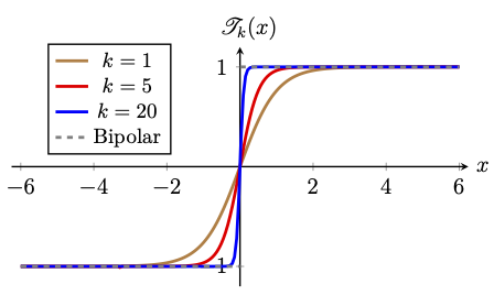
\[ \mathscr{T}_k(x) = \frac{e^{kx}-e^{-kx}}{e^{kx}+e^{-kx}},~x\in \mathbb{R}, k>0. \]

Graphs of the hyperbolic tangent function for various values of \(k\), illustrating convergence to the bipolar step function as \(k \to \infty\).

The graphs of the hyperbolic tangent function for various values of \(k\) are depicted in the above figure. From the figure, we observe that \(\mathscr{T}_k\rightarrow \mathscr{B}\) pointwise as \(k\rightarrow \infty\) on \(\mathbb{R}\backslash \{0\}\).

The hyperbolic tangent function is preferred over the bipolar function while learning an ANN using gradient-based optimization methods (such as gradient descent method).

Problem:

Show that \(\mathscr{T}_1 (x)=2\mathscr{S}_2(x)-1\).

The above problem shows that the tanh function is the logistic sigmoid stretched vertically (range doubled) and shifted downward by 1. Hence, the tanh activation function can be viewed as a particular affine transformation of the logistic sigmoid.

Bumped-type Functions

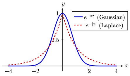
Bump functions are those which graphically resembles a bell-shaped curve, attains a maximum at some point, and decays rapidly to zero as \(x\rightarrow \pm \infty\).

For instance, the Gaussian bump \(\mathscr{G}_{\lambda,c}:\mathbb{R} \rightarrow (0,1]\), for fixed values of \(\lambda>0\) and \(c\in \mathbb{R}\), is defined as

\[ \mathscr{G}_{\lambda, c}(x) = e^{-\lambda(x-c)^2},~ x\in \mathbb{R}. \]

Another example of a bump function is the Laplace bump \(\mathscr{L}_{\lambda,c}: \mathbb{R} \rightarrow (0,1]\), for fixed values of \(\lambda>0\) and \(c\in \mathbb{R}\) and is defined as

\[ \mathscr{L}_{\lambda,c}(x) = e^{-\lambda|x-c|},~x\in \mathbb{R}, \]

which is not smooth. The graph of the Gaussian and Laplace bumps with \(\lambda=1\) and \(c=0\) are depicted in the following figure.

Graphs of the Gaussian and Laplace bumps with \(\lambda=1\) and \(c=0\).

Hockey-stick Functions

Any function whose graph resembles a hockey stick, i.e., an increasing L-shaped curve is a hockey-stick function.

Leaky Rectified Linear Unit

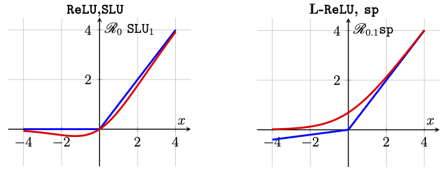
We are already familiar with the rectified linear unit from the first chapter (see the Example «Click Here» ). We now define a general form of this function, called the leaky rectified linear unit with parameter \(\alpha\in [0, 1)\) as the function \(\mathscr{R}_\alpha :\mathbb{R} \rightarrow \mathbb{R}\) defined as

\[ \mathscr{R}_\alpha(x) = \left\{\begin{array}{cc} \alpha x, & {if}~x<0,\\ x, & {if}~x\ge 0. \end{array}\right. \]

In particular, if we take \(\alpha=0\), we see that \(\mathscr{R}_0 = \texttt{ReLU}\) (see Example «Click Here»), which is the rectified linear unit defined as

\[ \mathscr{R}_0 (x) = \max\{0,x\},~x\in \mathbb{R}. \]

Many modern network models use \(\texttt{ReLU}\) as the activation function. This is mainly because the learning rate of a network involving \(\texttt{ReLU}\) is several times faster than networks with other sigmoid activation functions.

Instead of choosing \(\alpha\in [0,1)\), if we treate \(\alpha>0\) as a trainable parameter, then the activation function \(\mathscr{R}_\alpha\) is called the parametric rectified linear unit.

Sigmoid Linear Units

Sigmoid linear units (also called swish) is a smooth function \(\texttt{SLU}:\mathbb{R}\rightarrow \mathbb{R}\) defined as

\[ \texttt{SLU}_k(x) = x\mathscr{S}_k(x), \]

for a fixed parameter \(k>0\).

Problem:

Show that \(\texttt{SLU}_k(x) \rightarrow \texttt{ReLU}\)(x) as \(k\rightarrow \infty\), for all \(x\in \mathbb{R}\backslash \{0\}\).

Softplus Function

Another smooth version of the \(\texttt{ReLU}\) function is the softplus function defined as

\[ \texttt{sp}(x) = \text{ln}(1+e^x). \]

Problem:

Show the following properties:

\(\texttt{sp}(x) - \texttt{sp}(-x) = x.\)
\(\texttt{sp}'(x) = \mathscr{S}_1(x).\)

Graphs of hockey-stick functions are depicted in the following figure.

Graph of hockey-stick activation functions.

Multi-class Classification

Multi-class classification refers to assigning exactly one class to each input out of a set of more than two possible classes.

In a multi-class classification, the outputs (targets/labels) are often categories (discrete class names), such as identifying whether a photograph depicts a cat, or a dog, or a cow. In this case, the output is \(y \in \{\text{`cat'}, \text{`dog'}, \text{`cow'}\}.\)

Since neural networks cannot handle symbolic categories directly, the target must be represented numerically. A canonical way of interpreting an \(n\)-class classification numerically is to use one-hot vector encoding, where each class is represented by an \(n\)-dimensional vector \(\boldsymbol{e}_i=(0,0,\ldots,1,0,\ldots, 0)\), for \(i=1,2,\ldots, n\), with \(1\) appearing at the \(i^{\rm th}\) coordinate.

For instance, the above example is a 3-class classification, which can be encoded by the three dimensional one-hot mapping as

\begin{eqnarray} \text{`cat'} &\mapsto& (1,0,0)\\ \text{`dog'} &\mapsto& (0,1,0)\\ \text{`cow'} &\mapsto& (0,0,1) \end{eqnarray}

(4.13)

One-hot encoding is the canonical way to represent categorical targets in multi-class classification.

Softmax Function

In a multi-class classification problem with \(n\) classes, a neural network produces a pre-activation vector of real numbers at the output layer as

\[ \boldsymbol{z}=(z_1, z_2, \ldots, z_n)^\top, \]

whose entries are called the logits of the \(n\) classes.

To interpret these logits as probabilities of each class, we apply the softmax function as the activation function at the output layer to get the output as \(\boldsymbol{y} = (y_1, y_2, \ldots, y_n)^\top\), where

\[ y_i = \frac{e^{z_i}}{\displaystyle{\sum_{j=1}^n} e^{z_j}}, \text{ for } i=1,2,\ldots, n. \]

Thus, softmax is a function \(\texttt{sm}: \mathbb{R}^n \rightarrow \mathbb{R}^n\) defined by

\[ \texttt{sm}(\boldsymbol{z}) = \left( \frac{e^{z_1}}{\displaystyle{\sum_{i=1}^n} e^{z_i}}, \frac{e^{z_2}}{\displaystyle{\sum_{i=1}^n} e^{z_i}}, \ldots, \frac{e^{z_n}}{\displaystyle{\sum_{i=1}^n} e^{z_i}} \right),~\boldsymbol{z}\in \mathbb{R}^n. \]

The softmax plays the role of the logistic sigmoid in the multi-class setting in order to make the output vector \(\boldsymbol{y}\) a valid probability distribution over the \(n\) classes.

In the following example, we show that in the case of binary classification, the softmax reduces to the logistic sigmoid.

Example:

For logits \(\boldsymbol{z}=(z_1,z_2)\), the softmax gives

\[ y_1 = \frac{e^{z_1}}{e^{z_1}+e^{z_2}}, \qquad y_2 = \frac{e^{z_2}}{e^{z_1}+e^{z_2}}. \]

We can rewrite

\[ y_1 = \frac{1}{1+e^{z_2-z_1}} = \mathscr{S}_1(z_1-z_2),~ \text{and}~ y_2 = 1-y_1. \]

Thus, binary logistic regression is a special case of the softmax with two classes.

In general, for a given \(k>0\), we define the softmax as

\[ \texttt{sm}_k(\boldsymbol{z}) = \left( \frac{e^{kz_1}}{\displaystyle{\sum_{i=1}^n} e^{kz_i}}, \frac{e^{kz_2}}{\displaystyle{\sum_{i=1}^n} e^{kz_i}}, \ldots, \frac{e^{kz_n}}{\displaystyle{\sum_{i=1}^n} e^{kz_i}} \right),~\boldsymbol{z}\in \mathbb{R}^n. \]

Problem:

Show that \(\texttt{sm}_k(\boldsymbol{z}) \rightarrow \boldsymbol{e}_j\) as \(k\rightarrow \infty\), where \(j\in\{1,2,\ldots, n\}\) is such that \(z_j = \max\{z_1, . . . , z_n\}\).

Note:

For more details on activation functions refer to Section 2.1 (page 21) in the following book:

Calin, Ovidiu, Deep Learning Architectures: A Mathematical Approach, Springer, 2020.

Click here to see the details of the book