Perceptrons

In the previous chapter, we introduced the concept of an artificial neuron and outlined the supervised learning algorithm. Artificial neurons (ANs) are the building blocks for artificial neural networks (ANNs). A deeper understanding of ANs is therefore essential before proceeding further.

Perceptrons are the simplest and most fundamental among various types of artificial neurons. They are binary classifiers designed to classify datasets that are linearly separable, where the decision boundary is a hyperplane. In such cases, a simple learning algorithm can be devised to determine the model parameters. Moreover, convergence of the learning algorithm can be analyzed using simple mathematical arguments. This chapter is devoted to a detailed discussion on perceptrons that includes a multi-epoch perceptron learning algorithm and its convergence.

Section «Click Here» introduces perceptrons and illustrates the construction of perceptrons for certain Boolean functions. This section also includes the proof of the non-existence of a perceptron for the XOR function and motivates the notion of linear separability as a necessary and sufficient condition for the existence of a perceptron for a dataset. The mathematical notion of linear separability of a dataset is then introduced in Section «Click Here», where a discussion of the perceptron learning algorithm and a proof of the perceptron convergence theorem are presented. Finally, Section «Click Here» discusses the concept of feature mapping as a technique to handle datasets that are not linearly separable. We illustrate how mapping the input data to a higher-dimensional feature space can render it linearly separable, thereby enabling the construction of a perceptron in that feature space.

Neuron Model

The ancient and the simplest artificial neuron is the one with the activation function as the Heaviside function or the step function given by

\begin{eqnarray} H(x) = \left\{\begin{array}{lc} 0,&\text{if}~x<0\\ 1,&\text{if}~x\ge 0 \end{array}\right. \end{eqnarray}

(2.1)

Such an artificial neuron is called a perceptron, which we already illustrated in Example «Click Here» . Perceptrons are oversimplified models that resemble biological neuron, where if the weighted input exceeds a threshold or bias \(b\), then the neuron gets activated.

Note:

One can also use the bipolar step function as the activation function, which is defined as

\begin{eqnarray} H(x) = \left\{\begin{array}{rc} -1,&\text{if}~x<0\\ 1,&\text{if}~x\ge 0 \end{array}\right. \end{eqnarray}

(2.2)

Note that the perceptron theory we discuss here holds for both types of activation functions with some obvious modifications.

Remark:

We say that a perceptron exists for a given dataset \(\mathcal{D} = \{(\boldsymbol{x}_k, y_k)~|~k=1,2,\ldots, N\} \subset \mathbb{R}^n \times \{0, 1\}\) if there exists a \(\overline{\boldsymbol{w}}=(b,\boldsymbol{w}) \in \mathbb{R}\times \mathbb{R}^{n}\), where \(b\in \mathbb{R}\) is a bias and \(\boldsymbol{w}=(w_1,w_2,\ldots, w_n)\in \mathbb{R}^n\) is a weight vector, such that the resulting neuron \((\overline{\boldsymbol{w}}, H)\) exactly models the dataset. That is, the resulting neuron function \(\text{𝕗}\) satisfies \(\text{𝕗}(\boldsymbol{x}_k) = y_k\) for every \(k=1,2,\ldots, N\). Sometime, we also say that a perceptron can be learnt or trained if it exists for a dataset.

Boolean Functions

A Boolean function of \(n\) variables is a function that takes an \(n\)-dimensional input vector \(\boldsymbol{x}\in \{0,1\}^n\) and produces a binary output digit \(y\in \{0,1\}\).

Logical functions are examples of Boolean functions. Perceptrons can be used to represent some logical functions as illustrated below:

Example:

Consider the 2-dimensional dataset for logical AND function given in the following truth table:

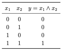It is straight forward to model a perceptron \((\overline{\boldsymbol{w}}, H)\) for the logical AND function. In fact, any choice of the weights \(w_1\) and \(w_2\), and the bias \(w_0=b\) such that

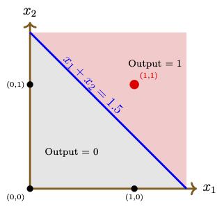
\[ b \left\{ \begin{array}{ll}< x_1w_1 + x_2 w_2 , &\text{if}~x_1=x_2=1\\ >x_1w_1 + x_2 w_2 , &\text{otherwise}. \end{array}\right. \]

will be a perceptron that generates the same output as the \(\land\) operator. Here the line \(x_1w_1 + x_2 w_2 = b\) is referred to as a decision boundary.

For instance, we can choose \(\overline{\boldsymbol{w}}=(1.5,1, 1)\). The figure below depicts the decision boundary \(x_1+x_2 = 1.5\) of the perceptron with the neuron function \(\text{𝕗}(x_1,x_2) = H(x_1+x_2-1.5).\)

Input vectors and decision boundary (blue) of a perceptron for the \(\land\) operator.

Problem:

Give the truth table for the OR gate function \(\lor: \{0,1\}^2\rightarrow \{0,1\}\). Considering the truth table as the dataset, provide the general form of a perceptron that models the OR function and give the corresponding neuron function. Choose a particular perceptron and draw the diagram in the \((x_1,x_2)\)-plane indicating the input data points, the decision boundary, and the regions corresponding to output values 0 and 1, for the chosen perceptron.

For \(n=2\), there are \( 2^4 = 16 \) possible Boolean functions. Each Boolean function \( f: \{0,1\}^2 \to \{0,1\} \) maps every pair \( (x_1, x_2) \) to either 0 or 1. The list of all Boolean functions are given in the following table. 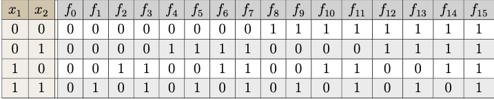Each column \( f_i \) corresponds to a Boolean function identified by the binary pattern in that column, interpreted as the output for inputs \((0,0), (0,1), (1,0), (1,1)\).

A few named Boolean functions are as follows:

\( f_0(x_1, x_2) = 0 \) (False)

\( f_1(x_1, x_2) = x_1 \land x_2 \) (AND)

\( f_6(x_1, x_2) = x_1 \oplus x_2 \) (XOR \(\rightarrow\) exclusive OR)

\( f_7(x_1, x_2) = x_1 \lor x_2 \) (OR)

\( f_8(x_1, x_2) = \neg (x_1 \lor x_2) \) (NOR)

\( f_9(x_1, x_2) = \neg (x_1 \oplus x_2) \) (XNOR)

\( f_{14}(x_1, x_2) = \neg (x_1 \land x_2) \) (NAND)

\( f_{15}(x_1, x_2) = 1 \) (True)

The following problem shows that not all Boolean functions can be represented by a perceptron.

Problem:

Show that there does not exist a perceptron for the XOR function.

Hint:

There are two ways in which we can prove the non-existence of a perceptron for the XOR function. One is a geometric approach, and the other is an algebraic approach. See page 139 in the following book:

Calin, Ovidiu, Deep Learning Architectures: A Mathematical Approach, Springer, 2020.

Click here to see the details of the book

Illustrative Datasets

The above problem shows that perceptrons cannot learn every dataset. More precisely, if the decision boundary in a dataset is not a hyperplane, then there does not exists a perceptron that exactly classifies the data.

In this subsection, we present two examples: one illustrating a linearly separable dataset which has a linear decision boundary, and another where the classes are not linearly separable.

We begin with a practical scenario where the data are separated by a linear decision boundary.

(a) The full dataset; (b) the training dataset for the example given below. Green dots indicate students who were successfully placed, while red dots represent those who were not placed. There are 250 examples in the full dataset and 70% of examples are taken randomly into the training dataset.

Example:

[ Placement Prediction System: Synthetic Dataset Generation]

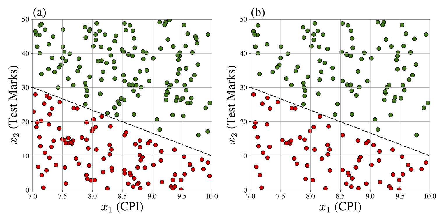
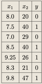
The placement office in an educational institute has a dataset of students who appeared for the placement for the past five years. Let us hypothetically assume that a student's success in getting a job depends only on the following two factors:

the CPI, denoted by \(x_1\); and
the marks scored in the screening test, denoted by \(x_2\).

The success in getting a job is denoted by \(y=1\) and the failure is taken as \(y=0\). The aim is to train a perceptron model to predict whether a student will get a job or not based on the values of \((x_1, x_2)\) of that student.

Recall that a perceptron is represented by the tuple \((\overline{\boldsymbol{w}}, H)\), where \(\overline{\boldsymbol{w}}=(b,w_1,w_2)\) is a weight vector to be obtained. Finding a weight vector \(\overline{\boldsymbol{w}}\) is referred to as learning (or training) a model. We have already outlined the learning algorithm for a neuron in the previous chapter. As per the learning algorithm, we first have to get a dataset \(\mathcal{D}_\text{train}\), called a training set, to train the model.

Assume that the placement office provided us with their dataset \(\mathcal{D}\), which is shown in Figure «Click Here» (a) and a training dataset \(\mathcal{D}_\text{train}\) is depicted in Figure «Click Here» (b). The decision boundary is shown as the black dashed line. Since the decision boundary is a straight line, we can train a perceptron for this dataset.

Code:

Understand the following python code that generates the above figure: PlacementPredictorDatasetGenerator

We will see in the next section that the dataset illustrated in the above example is a linearly separable dataset.

Our next example illustrates a practical scenario where the dataset is not linearly separable.

(a) The full dataset; (b) the training dataset for the example given below. Green dots represent approved applications and red dots indicate declined applications. There are 500 examples in the full dataset and 70% of examples are taken randomly into the training dataset.

Example:

[Credit Card Approval Decision System: Synthetic Dataset Generation]

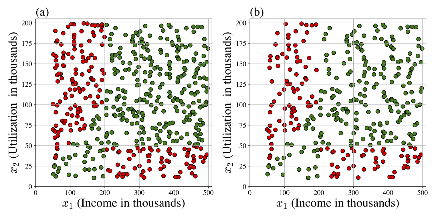
Assume that a bank issues credit cards, where they use various customer-related parameters for approval decisions. Over the years, the bank has accumulated a large database of credit card approval history, where humans were involved in taking the approval decisions based on certain internal policy rules. Now, the bank aims to build a model to automate these decisions.

For simplicity, let us assume that the approval decision depends only on two parameters, namely,

the customer's monthly income, denoted by \(x_1\); and
the customer's expected monthly expenditure through the credit card, denoted by \(x_2\).

Let us consider the bank's dataset \(\mathcal{D}\) as depicted in the above Figure «Click Here» (a). Further, a training dataset \(\mathcal{D}_\text{train}\) chosen randomly from \(\mathcal{D}\) is shown in the above Figure «Click Here» (b).

Code:

Write a Python code to plot a pair of figures similar to the above Figure «Click Here» by first generating a synthetic dataset \(\mathcal{D}\) and then randomly selecting 70% of the examples from \(\mathcal{D}\) to form a training dataset \(\mathcal{D}_\text{train}\).

Design your own decision boundary (that roughly resembles the observed boundary in the figure) by interpreting the following approval policy rules:

Customers with high income and high credit card utilization are approved.
Customers with low income and low credit card utilization are also approved.

Separability and Algorithm

In the previous section, we illustrated how to construct a perceptron for a given Boolean function. Since the datasets in those examples contained only a few data points, it was easy to obtain the weights manually, which we refer to as constructing a model. However, when the dataset is large, obtaining the weights manually may be computationally costly or even impossible. Therefore, it is desirable to have an efficient algorithm to compute the weights automatically. This can be achieved by first considering an appropriate cost function and then computing the weights that minimizes the cost function, which is referred to as learning a model. We discuss different ways of defining cost functions and some optimization methods in a later chapter. In this section, we introduce a simple learning algorithm to train a perceptron based on incremental updates.

Linear Separability

First, let us define the mathematical notion of a linearly separable dataset.

Definition:

[Linearly Separable]

Two subsets \(\mathcal{C}^-\) and \(\mathcal{C}^+\) of \(\mathbb{R}^{n}\) are said to be linearly separable if there exists a vector \(\overline{\boldsymbol{w}}=(w_0, w_1, \ldots, w_n) \in \mathbb{R}^{n+1}\) such that

\begin{eqnarray} \begin{array}{l} \text{for every } \boldsymbol{x}=(x_1, \ldots, x_n) \in \mathcal{C}^-, \text{ we have } \displaystyle{\sum_{k=1}^n} w_k x_k < w_0; {and}\\ \text{for every } \boldsymbol{x}=(x_1, \ldots, x_n) \in \mathcal{C}^+, \text{ we have } \displaystyle{\sum_{k=1}^n} w_k x_k \ge w_0. \end{array} \end{eqnarray}

(2.3)

We call such a vector \(\overline{\boldsymbol{w}}\) an augmented weight vector.

Remark:

[Geometric Interpretation]

Let us write the augmented weight vector as \(\overline{\boldsymbol{w}} = (w_0, \boldsymbol{w})\in \mathbb{R}\times \mathbb{R}^n\), where \(\boldsymbol{w}=(w_1,w_2,\ldots, w_n)\). If the sets \(\mathcal{C}^-\) and \(\mathcal{C}^+\) are linearly separable, then there exists a hyperplane

\[ L: \boldsymbol{w}\cdot\boldsymbol{x} = w_0, \]

called a decision boundary, that separates these two subsets. The weight vector \(\boldsymbol{w}\) is normal (perpendicular) to \(L\).

The following lemma provides a necessary and sufficient condition for the existence of a perceptron for a given dataset, which is a direct consequence of Remark «Click Here» and Definition «Click Here» .

Lemma:

[Existence of a Perceptron]

A perceptron exists for a dataset \(\mathcal{D}\subset \mathbb{R}^{n}\times \{0,1\}\) if and only if there exist two linearly separable sets \( \mathcal{C}^-\subset \mathbb{R}^{n}\) and \(\mathcal{C}^+\subset \mathbb{R}^{n} \) such that

\[ \mathcal{D} = \big(\mathcal{C}^- \times \{0\}\big) \cup \big(\mathcal{C}^+ \times \{1\} \big). \]

Remark:

While discussing neurons, we use the notation \(\mathcal{D} = \mathcal{C}\times \mathbb{R}\) to denote a dataset in supervised learning. Here, \(\mathcal{C}\) denotes the set of input vectors, and \(\mathbb{R}\) represents the corresponding outputs (or labels).

We call a dataset linearly separable if there exists a partition of the input set \(\mathcal{C}\) consisting of two linearly separable sets.

Equivalently, by virtue of Definition «Click Here» , we say that a dataset is linearly separable if there exists an augmented weight vector \(\overline{\boldsymbol{w}}\) that classifies all examples of the dataset correctly.

Training Algorithm

Given a linearly separable dataset, our next task is to design an algorithm that learns a perceptron by computing a separating hyperplane. We begin by describing an algorithm for a single epoch in the training process using a given training dataset \(\mathcal{D}_\text{train}\).

Algorithm:

[Perceptron Learning (Single Epoch)]

Input:

the training dataset
\[ \mathcal{D}_\text{train}=\{(\boldsymbol{x}_k,y_k)~|~ k=1,2,\ldots, N_\text{train}\}; \]
the initial augmented weight vector \(\overline{\boldsymbol{w}}_0=(b_0, w_{0,1}, \ldots, w_{0,n})\in \mathbb{R}^{n+1}\); and
the learning rate \(\eta \in (0,\infty)\).

Processing:

Let \(N_\text{train} = \#(\mathcal{D}_\text{train})\) (cardinality of the set \(\mathcal{D}_\text{train}\)).

For each \(k=1,2,\ldots, N_\text{train}\), perform the following perceptron update rule:

\[ \overline{\boldsymbol{w}}_k = \overline{\boldsymbol{w}}_{k-1} + \eta\Big( y_k - H(\overline{\boldsymbol{w}}_{k-1} \cdot \overline{\boldsymbol{x}}_k)\Big) \overline{\boldsymbol{x}}_k. \]

Recall, the augmented input vector is given by \(\overline{\boldsymbol{x}}_k = (-1, \boldsymbol{x}_k)\).

Output: \(\overline{\boldsymbol{w}}^{(1)} := \overline{\boldsymbol{w}}_{N_\text{train}}\).

Remark:

Observe from the above algorithm that the augmented weight vector \(\overline{\boldsymbol{w}}_N\) is obtained by sequentially applying the update rule to all the examples in the training dataset. Such a complete pass through the entire training set is referred to as an epoch.

Let us illustrate the computation of a single epoch by considering a small training dataset .

Example:

Consider the following training dataset \(\mathcal{D}_\text{train}\):

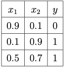Let us take \(\overline{\boldsymbol{w}}_0 = (0, 0, 0)\) and \(\eta = 1\).

Since our training dataset contains three examples (\(N_{\text{train}}=3\)), we have to perform three updates to obtain the augmented weight vector \(\overline{\boldsymbol{w}}^{(1)}\) in one epoch.

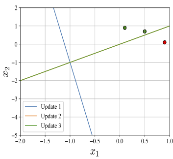
The updates in a single epoch using Algorithm «Click Here» are the following:

Update 1: \(\overline{\boldsymbol{w}}_1 = (1,-0.9,-0.1).\)

Update 2: \(\overline{\boldsymbol{w}}_2 = (0, -0.8, 0.8).\)

Update 3: \(\overline{\boldsymbol{w}}_3 = (0, -0.8, 0.8).\)

Therefore, the augmented weight vector after the single epoch is given by

\[ \overline{\boldsymbol{w}}^{(1)} = (0, -0.8, 0.8). \]

The perceptron learnt from the single epoch Algorithm «Click Here» is \((\overline{\boldsymbol{w}}^{(1)},H)\). The decision lines along with the training dataset are depicted in the following figure.

Decision lines for the updates in Example «Click Here» .

Problem:

Perform one epoch for the following training dataset \(\mathcal{D}_\text{train}\) with \(\overline{\boldsymbol{w}}_0 = (0, 0, 0)\) and \(\eta = 1\) to obtain the augmented weight vector \(\overline{\boldsymbol{w}}^{(1)}\):

Test the perceptron model (\(\overline{\boldsymbol{w}}^{(1)},H)\) on the training set by directly applying the model to each example of the dataset. Give the conclusion about whether the trained perceptron represents the training dataset exactly or not.

Code:

Understand the following Python code implementing Algorithm «Click Here» :

SingleEpochPerceptron

Modify the above Python code to include a visual representation (graph) of the given dataset along with the graph of the separating lines at each update.

The datasets considered in the following problem is similar to the placement prediction problem considered in Example «Click Here» .

Problem:

Consider the training dataset \(\mathcal{D}_\text{train}\) given in the following table:

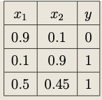
Take \(\overline{\boldsymbol{w}}_0=\boldsymbol{0}\), the zero vector, and \(\eta=0.9\). Perform one epoch to get \(\overline{\boldsymbol{w}}^{(1)}\) using Algorithm «Click Here» . Does the perceptron model \((\overline{\boldsymbol{w}}^{(1)}, H)\) fit the training dataset exactly?

Often, a single epoch is not sufficient to obtain a perceptron that exactly (or even approximately) fits the training dataset. In such cases, it is necessary to perform multiple epochs, by taking the output of one epoch as the initial weight vector for the next epoch, and updating the weights iteratively until a satisfactory perceptron is learned.

The following algorithm trains a perceptron using multiple epochs:

Algorithm:

[Perceptron Learning (Multiple Epoch)]

Input:

the training dataset \(\mathcal{D}_\text{train}=\{(\boldsymbol{x}_k,y_k)~|~ k=1,2,\ldots, N_\text{train}\}\);
the initial augmented weight vector \(\overline{\boldsymbol{w}}_0=(b_0, w_{0,1}, \ldots, w_{0,n})\in \mathbb{R}^{n+1}\); and
the learning rate \(\eta \in (0,\infty)\).

Processing: Let \(N_\text{train} = \#(\mathcal{D}_\text{train})\) (cardinality of the set \(\mathcal{D}_\text{train}\))

Set \(\overline{\boldsymbol{w}}^{(0)} = \overline{\boldsymbol{w}}_0.\)
Define the augmented input vector \(\overline{\boldsymbol{x}}_k = (-1, \boldsymbol{x}_k)\), for all \(k=1,2,\ldots, N_\text{train}\).
For each \(j=1,2,\ldots\), perform the following single epoch:
Update: For each \(k=1,2,\ldots, N_\text{train}\), perform the following update rule:
Step 1: Compute \(\Delta_k = y_k - H(\overline{\boldsymbol{w}}_{k-1} \cdot \overline{\boldsymbol{x}}_k).\)
Step 2: If \(| \Delta_k| < 1\), then take \(\overline{\boldsymbol{w}}_k = \overline{\boldsymbol{w}}_{k-1}.\)
Step 3: Otherwise, use the perceptron update rule:
\[ \overline{\boldsymbol{w}}_k = \overline{\boldsymbol{w}}_{k-1} + \eta\Delta_k\, \overline{\boldsymbol{x}}_k. \]
Assign: Set \(\overline{\boldsymbol{w}}^{(j)} := \overline{\boldsymbol{w}}_{N_\text{train}}\).
Check: For \(j\ge 1\), check the following condition:
\begin{eqnarray} \|\overline{\boldsymbol{w}}^{(j)} - \overline{\boldsymbol{w}}^{(j-1)}\|_2 = 0. \end{eqnarray}
(2.4)
If this condition is not satisfied, then take \(\overline{\boldsymbol{w}}_0 = \overline{\boldsymbol{w}}_{N_\text{train}}\) and go for the next epoch (Point 3 above).
Else if this condition is satisfied, then stop the computation.

Output: \(\overline{\boldsymbol{w}}^{(n_e)}\) where \(n_e=j-1\), the number of epochs taken to get a desired weight.

Note:

The norm \(\|\cdot\|_2\) used in the check condition above is the euclidean norm.

Remark:

[Perceptron Convergence]

If the check condition in the above algorithm is satisfied for some \(j=1,2,\ldots\), we say that the perceptron algorithm converged in \(j-1\) epochs.

The perceptron trained through the above multi-epoch algorithm is denoted by \((\overline{\boldsymbol{w}}^{(n_e)}, H)\), where \(n_e\) denotes the number of epochs taken by the algorithm to converge.

Code:

Extend the python program given in Code «Click Here» to implement the multiple epoch perceptron learning Algorithm «Click Here» . Test your code with the following dataset:

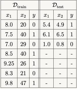Take \(\overline{\boldsymbol{w}}=\boldsymbol{0}\), the zero vector, and \(\eta=0.9\). Find the number of epochs needed for the convergence of the weight vector sequence. Let the weight vector limit be \(\overline{\boldsymbol{w}}^{*}\). Using the perceptron model \((\overline{\boldsymbol{w}}^{*}, H)\), compute the mean squared error on the test dataset.

Problem:

For a given \(\overline{\boldsymbol{w}}^{(0)}\), \(\eta>0\) and a training set \(\mathcal{D}_\text{train}\), let \(\{\overline{\boldsymbol{w}}^{(j)} \mid j = 1, 2, \ldots\}\) be a sequence generated by the multi-epoch Algorithm «Click Here» . Suppose that there exists an integer \(J\ge 0\) such that the perceptron \((\overline{\boldsymbol{w}}^{(J)}, H)\) correctly classifies all the examples of the training dataset \(\mathcal{D}_\text{train}\). Then, show that the algorithm converges in \(n_e = J\) epochs. Does the converse hold? Justify your answer.

Perceptron Convergence Theorem

The following theorem provides a sufficient condition for the convergence of the multi-epoch Algorithm «Click Here» in finite epochs.

Theorem:

[Perceptron Convergence Theorem]

Let the training dataset \(\mathcal{D}_\text{train}=\{(\boldsymbol{x}_k,y_k)~|~ k=1,2,\ldots, N_\text{train}\}\) be linearly separable, and let \(\overline{\boldsymbol{w}}^*\) be an augmented weight vector such that the perceptron \((\overline{\boldsymbol{w}}^*, H)\) classifies all examples of \(\mathcal{D}_\text{train}\) correctly with \(\overline{\boldsymbol{w}}^*\cdot \overline{\boldsymbol{x}}_k \ne 0\), for all \(k=1,2,\ldots, N_\text{train}\). Then, for any initial augmented vector \(\overline{\boldsymbol{w}}_0\) such that \(\overline{\boldsymbol{w}}^*\cdot \overline{\boldsymbol{w}}_0\ge 0\) and any learning rate \(\eta > 0\), there exists an integer \(n_e\ge 0\) such that the perceptron \((\overline{\boldsymbol{w}}^{(n_e)}, H)\) classifies all examples in \(\mathcal{D}_\text{train}\) correctly, where \(\overline{\boldsymbol{w}}^{(n_e)}\) is computed using the multi-epoch Algorithm «Click Here» .

Proof:

Assume the contrary that the multi-epoch perceptron Algorithm «Click Here» performs epochs indefinitely.

Assume that the multi-epoch perceptron Algorithm «Click Here» had performed \(n_e>0\) number of epochs and not all examples are correctly classified by the vector \(\overline{\boldsymbol{w}}^{(n_e) }\). Further, assume that \(\overline{\boldsymbol{w}}^{(n_e) }\) is obtained after \(m-1\) updates.

Let \(k_1\in \{1,2,\ldots, N_\text{train}\}\) be the smallest integer such that the example (\(\boldsymbol{x}_{k_1}, y_{k_1}\)) is not classified correctly by \(\overline{\boldsymbol{w}}^{(n_e) }\). Then, the algorithm performs the \(m^\text{th}\) update and obtains \(\overline{\boldsymbol{w}}_{m}\) which satisfies (how?)

\[ \overline{\boldsymbol{w}}^*\cdot \overline{\boldsymbol{w}}_{m} \ge \overline{\boldsymbol{w}}^*\cdot\overline{\boldsymbol{w}}_0 + m\eta \rho. \]

where

\[ \rho = \min\Big\{|\overline{\boldsymbol{w}}^*\cdot \overline{\boldsymbol{x}}_k|~|~ k=1,2,\ldots, N_\text{train}\Big\}>0.\\ \]

Using Cauchy-Schwarz inequality, we obtain

\begin{eqnarray} \|\overline{\boldsymbol{w}}_{m}\|^2 \ge \frac{\big( \overline{\boldsymbol{w}}^*\cdot\overline{\boldsymbol{w}}_0 + m\eta \rho \big)^2}{\|\overline{\boldsymbol{w}}^*\|^2}. \end{eqnarray}

(2.5)

On the other hand, since \(\overline{\boldsymbol{x}}_{k_1}\) is not classified by \(\overline{\boldsymbol{w}}_{m-1}\) correctly, we can show that (how?)

\begin{eqnarray} \|\overline{\boldsymbol{w}}_{m}\|^2 \le \|\overline{\boldsymbol{w}}_{0}\|^2 + m\eta^2 r^2. \end{eqnarray}

(2.6)

where \(r := \max\{\|\overline{\boldsymbol{x}}_{k}\|~|~k=1,2,\ldots, N_\text{train}\}\). The above two inequalities leads to a contradiction to our assumption that the algorithm performs epochs indefinitely. Thus, the algorithm has to terminate in a finite number of epochs.

Further, by equating the lower and the upper bounds of \(\|\overline{\boldsymbol{w}}_{m}\|^2 \), we can obtain the maximum number of updates, denoted by \(m^*>0\) (justify the existence of a positive \(m^*\)). If there is an example \(\overline{\boldsymbol{x}}_k\) that has still not been classified correctly by \(\overline{\boldsymbol{w}}_{m^*}\), then the algorithm will proceed to the next update \(\overline{\boldsymbol{w}}_{m^*+1}\), which must satisfy the above two conditions. But, both these conditions do not hold simultaneously for \(m=m^*+1\) (why?). Therefore, the perceptron (\(\overline{\boldsymbol{w}}_{m^*},H)\) has to classify all the examples correctly.

Note:

Note the difference between the number of epochs and the number of updates, as is apparent from the above proof.

Beyond Linear Separability

In the previous section, we discussed a simple multi-epoch algorithm to train a perceptron to classify a linearly separable dataset. However, in real-world applications, we often encounter datasets that are not linearly separable.

There are two main scenarios where linear separability does not hold in a dataset:

When the decision boundary cannot be represented by a hyperplane (for example, circular or any curved decision boundaries). In such cases, the dataset is said to be nonlinearly separable and the decision boundary is called the nonlinear discriminants.
When the classification task require multiple hyperplanes (or curved surfaces) to separate the classes. This occurs in problems with complex class structures (such as the XOR example discussed in Problem «Click Here» and the dataset generated in the credit card approval Example «Click Here» ) or multi-class classification problems.

The perceptron learning algorithm is only guaranteed to converge when the dataset is linearly separable. In general, single-neuron models are insufficient to learn datasets with complex decision boundaries. There are at least two broad approaches to handle this situation. One is to combine multiple neurons with nonlinear activation functions to form a deep neural network, which will be the subject of discussion in later chapters. The other involves alternative machine learning tool called feature engineering, which we will briefly explore in this section.

The underlying idea of feature engineering is to transform the input data into another space, called the feature space, where the dataset becomes linearly separable. In this section, we discuss the feature space transformation with a few illustrations.

Feature Space Mapping

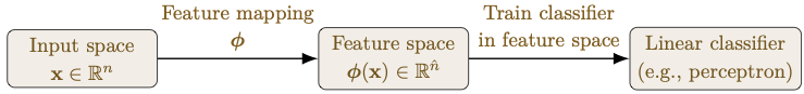
Even if a dataset is not linearly separable in the input space, it may be possible to transform the input vectors \(\boldsymbol{x} \in \mathbb{R}^n\) into new representations \(\boldsymbol{\phi}(\boldsymbol{x}) \in \mathbb{R}^{\hat{n}}\), such that the equivalent transformed dataset becomes linearly separable. The perceptron training Algorithm «Click Here» can then be applied directly in the feature space to learn a linear classifier for the transformed data (see the following figure).

Schematic view of mapping input data to a feature space where a linear classifier can be applied.

The function \(\boldsymbol{\phi}:\mathbb{R}^n\rightarrow \mathbb{R}^{\hat{n}}\), with \(\hat{n}\ge n\), is a nonlinear map called the feature function. It maps the input space \(\mathbb{R}^n\) into a feature space \(\mathbb{R}^{\hat{n}}\).

We write \(\boldsymbol{\phi}(\boldsymbol{x}) = (\phi_1(\boldsymbol{x}), \phi_2(\boldsymbol{x}), \ldots, \phi_{\hat{n}}(\boldsymbol{x}))\), where each component \(\phi_k:\mathbb{R}^n\rightarrow \mathbb{R}\), for \(k=1,2,\ldots, \hat{n}\), is called a basis function.

Consider the augmented feature function \(\overline{\boldsymbol{\phi}}(\boldsymbol{x}) = (-1, \phi_1(\boldsymbol{x}), \phi_2(\boldsymbol{x}), \ldots, \phi_{\hat{n}}(\boldsymbol{x}))\) and define the generalized linear discriminant as

\[ \text{𝕒}(\overline{\boldsymbol{\phi}}(\boldsymbol{x});\overline{\boldsymbol{w}}) = \sum_{k=0}^{\hat{n}} w_k \phi_k(\boldsymbol{x}) = \sum_{k=1}^{\hat{n}} w_k \phi_k(\boldsymbol{x}) - b, \]

for a given augmented weight vector \(\overline{\boldsymbol{w}}=(w_0,w_1,\ldots, w_{\hat{n}})\) in the feature space \(\mathbb{R}^{\hat{n}}\) with \(w_0=b\in \mathbb{R}\) being the bias.

If such a feature map is constructed, then a neuron (such as a perceptron) can be trained on this transformed dataset using a linear classifing algorithm (such as the perceptron Algorithm «Click Here» ).

To have a better understanding of the feature space transformation, we illustrate the construction of feature maps for a given dataset provided the discriminant function is known explicitly.

Example:

[Circular Decision Boundary]

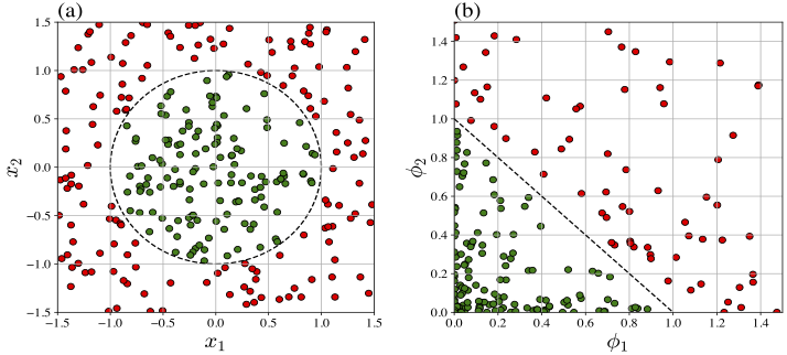
Consider a two-dimensional input \( \boldsymbol{x} = (x_1, x_2) \). Let the nonlinear discriminant function in the input space be

\[ \text{𝕒}(\boldsymbol{x}) = x_1^2 + x_2^2 - r^2, \]

where \( r > 0 \) is a given real number. The function \(\text{𝕒}\) is nonlinear since it defines a circular decision boundary \(x_1^2 + x_2^2 = r^2\), where the region inside the circle corresponds to \(\text{𝕒}(\boldsymbol{x}) < 0 \), and the region outside corresponds to \(\text{𝕒}(\boldsymbol{x}) \ge 0 \).

In particular, consider the training dataset \(\mathcal{D}_{\text{train}} = \{(\boldsymbol{x}_k, y_k)\} \subset \mathbb{R}^2\times \{0,1\}\) depicted in Figure «Click Here» (a). Here, we have taken \(r=1\) and the decision boundary is the unit circle. Obviously, Algorithm «Click Here» cannot be used to train a perceptron that represents this dataset correctly.

However, by mapping the training dataset into a suitable chosen feature space, we can train a perceptron. For instance, choose \(\boldsymbol{\phi}(x_1,x_2) = (x_1^2, x_2^2)\), where the basis functions are \(\phi_k(x_1,x_2) = x_k^2\), \(k=1,2\). Then, we can see that the generalized linear discriminant is

\[ \text{𝕒} = \overline{\boldsymbol{w}}\cdot \overline{\boldsymbol{\phi}}, \]

where the augmented weight vector is \(\overline{\boldsymbol{w}} = (r^2, 1, 1)\) and the augmented feature function is \(\overline{\boldsymbol{\phi}}=(-1, \phi_1, \phi_2)\). Algorithm «Click Here» can then be applied on the dataset in the \((\phi_1, \phi_2)\)-plane, which is the feature space. The training dataset \(\mathcal{D}_{\text{train}} = \{(\boldsymbol{\phi}_k, y_k)\}\) in the feature space is depicted in Figure «Click Here» (b).

An illustration of a nonlinearly separable dataset mapped to a linearly separable dataset with feature map discussed in Example «Click Here» . Here, red dots represent labels with value \(0\) and green dots correspond to labels with value +1. Black dashed line represents the decision boundaries in the respected spaces. (a) Dataset in the input space (b) Dataset in the feature space.

In the previous example, we illustrated an exact construction of the discriminant function, which is possible because the given function is a polynomial. However, if the discriminant function is non-polynomial, an explict feature space mapping may not be feasible. In this case, we have to approximate the discriminant function. We illustrate such a situation in the following problem.

Problem:

Let the training dataset \(\mathcal{D}_\text{train}\in \mathbb{R}^2\times \{0,1\}\) be such that the discriminant function is given by

\[ \text{𝕒}(x_1, x_2)=e^{x_1^2 + x_2^2}. \]

Using the Taylor expansion of \(\text{𝕒}\) about the origin up to total degree 4, construct a feature mapping function \(\boldsymbol{\phi} : \mathbb{R}^2 \rightarrow \mathbb{R}^{\hat{d}}\) such that the dataset, when mapped into the feature space \(\mathbb{R}^{\hat{d}}\), can be separated by a linear discriminant function. Also, obtain a suitable weight vector \(\boldsymbol{w}\).

Partial Answer: \(\hat{d} = 6\)

Recall, in Problem «Click Here» , we have seen that it is not possible to train a perceptron for the XOR function in the input space. However, by suitably choosing a feature map, we can train a perceptron for XOR in the feature space.

Problem:

Obtain a suitable feature map \(\boldsymbol{\phi}\) such that the XOR function \( f_6(x_1, x_2) = x_1 \oplus x_2 \) is represented exactly by a perceptron in the feature space.

Building a feature map explicitly is seldom feasible, as the discriminant function is typically unknown and implicitly embedded in the dataset. It is therefore desirable to adapt methodologies in which the feature map is learned as part of the training process. This is a core idea in deep learning, where multiple layers of artificial neurons are used to extract increasingly abstract features from data. However, there are also other well-established machine learning models, such as Support Vector Machines (SVMs), that can learn complex decision boundaries directly from data through the use of kernels, without requiring an explicit construction of the feature map.